
Chapter 6
THE LOW-ORDER METHOD (ILOWHI=0)
This Chapter includes specific topics which are applicable when the low-order method is used, as in earlier versions of WAMIT. The essential features of this method are (a) the geometry of the body is represented by an ensemble of flat quadrilateral panels, or facets, and (b) the solutions for the velocity potential, and optionally for the source strength, are approximated by piecewise constant values on each panel.
The geometry of the body is specified in this case by a Geometric Data File (GDF) which includes the Cartesian coordinates of each vertex of each panel, listed sequentially. In addition the GDF file specifies the characteristic length ULEN used for nondimensionalization of outputs, the value of the gravitational acceleration constant GRAV in the same units of measurement, the number of panels NPAN, and two symmetry indices ISX, ISY, as described in Section 6.1. The syntax for data in this file follows the same requirements outlined for the generic input files in Chapter 4.
When the low-order method is used there are two different solutions which can be used, referred to as the potential source formulations. The potential formulation, which is always evaluated, represents the velocity potential in terms of surface distributions of sources and normal dipoles (See Section 15.2). This is used to evaluate hydrodynamic quantities including the first-order pressure, force coefficients and drift forces based on momentum conservation (Option 8). For the evaluation of these outputs the potential formulation is more general and efficient.
The source formulation is optional, depending on the configuration parameter ISOR (See Section 4.7). In the source formulation the potential is represented by a surface distribution of sources only, as explained in Section 15.3. The source formulation must be used if the mean drift force and moment are evaluated by pressure integration, also in some cases where the drift forces are evaluated using control surfaces (Chapter 11), and more generally if the fluid velocity is required on the body surface. The procedure for including the source formulation is used is described in Section 6.2.
If the body has thin elements, there are two possible approaches. The first is to panel both sides of these elements, with a finite thickness to separate the two sides. The disadvantage of this approach is that, as a general rule, the size of the panels must be comparable to the thickness, and thus a very large number of small panels may be required to achieve accurate results. The second approach is to reduce the thickness to zero, and represent the corresponding elements of the body by special ‘dipole panels’. This approach is analogous to the thin-wing approximation in lifting-surface theory [21]. WAMIT permits the user to specify a set of dipole panels, as described in Section 6.3. This option facilitates the analysis of bodies with damper plates, strakes, and similar thin elements, without the need to use very large numbers panels or to artificially increase the thickness.
6.1 THE GEOMETRIC DATA FILE
In the low-order method the wetted surface of a body is represented by an ensemble of connected four-sided facets, or panels. The Geometric Data File contains a description of this discretized surface, including the body length scale, gravity, symmetry indices, the total number of panels specified, and for each panel the Cartesian coordinates x,y,z of its four vertices. A panel degenerates to a triangle when the coordinates of two vertices coincide. The order in which the panels are defined in the file is unimportant, but each panel must be described completely by a set of 12 real numbers (three Cartesian coordinates for each vertex) which are listed consecutively, with a line break between the last vertex of each panel and the first vertex of the next. The value of gravity serves to define the units of length, which apply to the body length scale, panel offsets, and to all related parameters in the other input files. The coordinate system x,y,z in which the panels are defined is referred to as the body coordinate system. The only restrictions on the body coordinate system are that it is a right-handed Cartesian system and that the z-axis is vertical and positive upward.
The name of the GDF file can be any legal filename accepted by the operating system, with a maximum length of 16 ASCII characters, followed by the extension ‘.gdf’.
The data in the GDF file can be input in the following form:
ULEN GRAV
ISX ISY
NPAN
X1(1) Y1(1) Z1(1) X2(1) Y2(1) Z2(1) X3(1) Y3(1) Z3(1) X4(1) Y4(1) Z4(1)
X1(2) Y1(2) Z1(2) X2(2) Y2(2) Z2(2) X3(2) Y3(2) Z3(2) X4(2) Y4(2) Z4(2)
.
.
.
. . . . . . . . . . . . X4(NPAN) Y4(NPAN) Z4(NPAN)
Each line of data indicated above is input by a separate FORTRAN READ statement, hence line breaks between data must exist as shown. Additional line breaks between data shown above have no effect on the READ statement, so that for example the user may elect to place the twelve successive coordinates for each panel on four separate lines. (However the format used above is more efficient regarding storage and access time.)
Input data must be in the order shown above, with at least one blank space separating data on the same line.
The definitions of each entry in this file are as follows:
‘header’ denotes a one-line ASCII header dimensioned CHARACTER*72. This line is available for the user to insert a brief description of the file, with maximum length 72 characters.
ULEN is the dimensional length characterizing the body dimension. This parameter corresponds to the quantity L used in Chapter 4 to nondimensionalize the quantities output from WAMIT. ULEN can be input in any units of length, meters or feet for example, as long as the length scale of all other inputs is in the same units. ULEN must be a positive number, greater than 10-5. An error return and warning statement are generated if the last restriction is not satisfied.
GRAV is the acceleration of gravity, using the same units of length as in ULEN. The units of time are always seconds. If lengths are input in meters or feet, input 9.80665 or 32.174, respectively, for GRAV.
ISX, ISY are the geometry symmetry indices which have integer values 0, +1. If ISX and/or ISY =1, x = 0 and/or y = 0 is a geometric plane of symmetry, and the input data (panel vertex coordinates X,Y,Z and their total number NPAN) are restricted to one quadrant or one half of the body, namely the portion x > 0 and/or y > 0. Conversely, if ISX=0 and ISY=0, the complete submerged surface of the body must be represented by panels.
ISX = 1: The x = 0 plane is a geometric plane of symmetry.
ISX = 0: The x = 0 plane is not a geometric plane of symmetry.
ISY = 1: The y = 0 plane is a geometric plane of symmetry.
ISY = 0: The y = 0 plane is not a geometric plane of symmetry.
For all values of ISX and ISY, the (x,y) axes are understood to belong to the body system. The panel data are always referenced with respect to this system, even if walls or other bodies are present.
NPAN is equal to the number of panels with coordinates defined in this file, i.e. the number required to discretize a quarter, half or the whole of the body surface if there exist two, one or no planes of symmetry respectively.
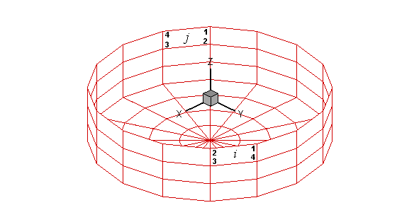
X1(1), Y1(1), Z1(1) are the (x,y,z) coordinates of vertex 1 of the first panel, X2(1), Y2(1), Z2(1) the (x,y,z) coordinates of the vertex 2 of the first panel, and so on. These are expressed in the same units as the length ULEN. The vertices must be numbered in the counter-clockwise direction when the panel is viewed from the fluid domain, as shown in Figure 6.1. The precise format of each coordinate is unimportant, as long as there is at least one blank space between coordinates, and the coordinates of the four vertices representing a panel are listed sequentially.
There are two situations when panels lie on the free surface, and thus all four vertices are on the free surface: (1) the discretization of a structure which has zero draft over part or all of its submerged surface, and (2) the discretization of the interior free surface for the irregular frequency removal as described in Chapter 10. For the first case, where the panels are part of the physical surface, the panel vertices must be numbered in the counter-clockwise direction when the panel is viewed from the fluid domain as in the case of submerged panels. For the second case, where the panel is interior to the body and non physical, the vertices must be numbered in the clockwise direction when the panel is viewed from inside the structure (or in the counter-clockwise direction when the panel is viewed from above the free surface). Details of the discretization of the interior free surface are provided in Chapter 10.
Although the panels on the free surface are legitimate in these two special cases, a warning message is displayed by WAMIT when it detects panels with zero draft, which have four vertices on the free surface. This is to provide a warning to users for a possible error in the discretization other than the above two exceptional cases. The run continues in this case, without interruption. An error message is displayed with an interruption of the run when the panels have only three vertices on the free surface, unless two adjacent vertices are coincident. (The latter provision permits the analysis of a triangular panel with one side in the free surface.)
The three Cartesian coordinates of four vertices must always be input for each panel, in a sequence of twelve real numbers. Triangles are represented by allowing the coordinates of two adjacent vertices to coincide, as in the center bottom panels shown in Figure 6.1. Two adjacent vertices are defined to be coincident if their included side has a length less than ULEN × 10-6. An error return results if the computed area of any panel is less than ULEN2 × 10-10.
The input vertices of a panel do not need to be co-planar. WAMIT internally defines planar panels that are a best fit to four vertices not lying on a plane. However it is advisable to discretize the body so that the input vertices defining each panel lie close to a plane, in order to achieve good accuracy in the computed velocity potentials. An error message is printed if a panel has two intersecting sides. A warning message is printed if a panel is ‘convex’ (the included angle between two adjacent sides exceeds 180 degrees).
The origin of the body coordinate system may be on, above or below the free surface. The vertical distance of the origin from the free surface is specified in the Potential Control File. The same body-system is also used to define the forces, moments, and body motions. (See Chapter 5 regarding the change in reference of phase relations when walls are present.)
Only the wetted surface of the body should be paneled, and then only half or a quarter of it if there exist one or two planes of symmetry respectively. This also applies to bodies mounted on the sea bottom or on one or two vertical walls. The number of panels NPAN refers to the number used to discretize a quarter, half or the whole body wetted surface if two, one or no planes of symmetry are present respectively.
The displaced volume of the structure deserves particular discussion. Three separate algorithms are used to evaluate this quantity, as explained in Section 3.1. Except for the special case where the structure is bottom-mounted, the three evaluations (VOLX, VOLY, VOLZ) should be identical, but they will generally differ by small amounts due to inaccuracies in machine computation and, more significantly, to approximations in the discretization of the body surface.
A general-purpose pre-processor has been developed for preparation of GDF files, using the MultiSurf geometric modelling program.1
6.2 USE OF THE SOURCE FORMULATION (ISOR=1)
This section describes the evaluation and use of the source strength, in the context of calculating the fluid velocity components on the body and the mean drift force and moment based on pressure integration in uni- and bi-directional waves.
In order to evaluate effectively the tangential components of the fluid velocity on the body (and hence the second-order mean pressure), the solution for the velocity potential based on Green’s theorem is augmented if ISOR=1 by the corresponding solution for the source distribution on the body surface. A brief description of the theory is provided in Section 15.4. (Further details are given in [10] and [26].)
Setting the parameter ISOR=1 in the configuration files specifies that the source-distribution integral equation is solved in addition to the velocity-potential integral equation. This is required in some cases for Options 5,6,7 and 9 in the FRC file, as noted in Section 4.3.
Values of the drift force and moment can be compared with the corresponding outputs evaluated using momentum conservation (Option 8), and with the drift forces evaluated using the control surface (Option 7). In general the results obtained from integration of the second-order pressure will require a finer discretization on the body surface, particularly in the vicinity of sharp corners.
Body symmetries can be exploited to minimize computing time. Special attention must be given to the evaluation of the drift forces, since these are dependent on quadratic products of the first-order solution. For example, if the body has two planes of symmetry the vertical first-order exciting force and heave response can be evaluated simply by setting IRAD=-1, IDIFF=0, MODE(3)=1, and the remaining MODE indices equal to zero. This will not give the correct vertical drift force on the body, however, since the components of the diffraction potential and body motions which are odd functions of x and y have not been evaluated. In general the drift forces should be evaluated only after evaluating all components of the first-order potential, i.e. by setting IDIFF=1 for the stationary body and IRAD=1 and IDIFF=1 for the freely floating body in the POT file. [An example of a valid short cut exists if both the body geometry and the hydrodynamic flow field are symmetrical about a plane of symmetry; then it is not necessary to evaluate first-order potentials which are odd about that plane since these would vanish. For example, if the body is symmetrical about y = 0 and the incident-wave heading angle is either zero or 180∘, the drift force and moment can be obtained by setting MODE(n)=0 for n = 2, 4, 6.]
To calculate the mean drift forces it is necessary to evaluate the runup or, equivalently, the velocity potential at the waterline. Since the program utilizes the velocity potentials at the centroids of the panels adjacent to the waterline for the runup, it is advisable to use panels with small vertical dimensions near the waterline.
6.3 BODIES WITH THIN SUBMERGED ELEMENTS
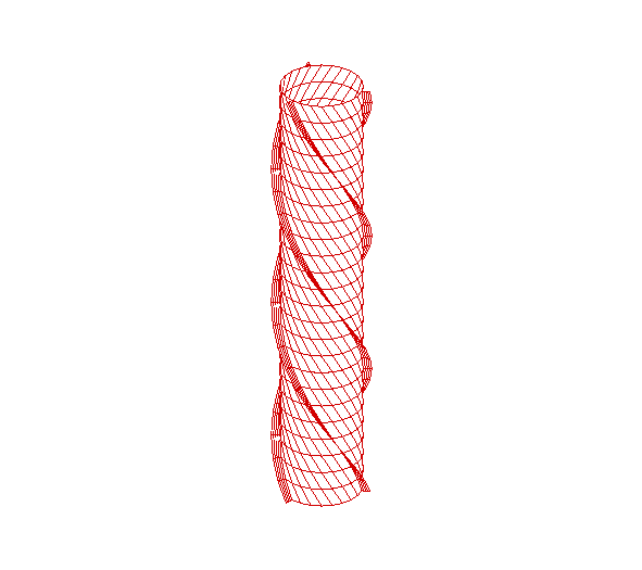
Bodies which consist partially (or completely) of elements with small or zero thickness can be analysed by defining these elements as ’dipole panels’. The geometry of these elements is represented by panels in the same manner as conventional body panels (Section 6.1). Figure 6.2 shows a typical example of a floating spar with thin helical strakes. This structure is analyzed in Test Run 09, described in the Appendix (Section A.9).
The velocity potential on the dipole panels is represented by dipoles alone, with no corresponding sources. The unknown is the difference of the velocity potential on the two sides, which is proportional to the pressure jump across the panel. Since both sides of the dipole panels adjoin the fluid, the direction of the normal vector is irrelevant. A positive difference of the velocity potential is defined to act in the normal direction to the surface from the side on which the vertices are in the counter-clockwise direction to the opposite side. The order of the vertices in the GDF file is arbitrary, as long as they are in a logical sequence to form a closed quadrilateral with contiguous sides.
The indices of the dipole panels are defined in the CFG file by including one or more lines starting with ‘NPDIPOLE=’, followed by the indices or ranges of indices of the dipole panels, as explained in Section 4.7. In this case the format of the GDF file is as explained for the case without dipole panels in Section 6.1, and the parameter NPAN is the total number of panels including both conventional and dipole types. The dipole panels may be located arbitrarily within the array of all panels. It is possible to analyze bodies which consist entirely of zero-thickness elements, by including the line ‘NPDIPOLE= (1 nn)’ in the CFG file, where nn=NPAN is the same integer value input in the GDF file.
The source formulation cannot be used if dipole panels are included. Thus the fluid velocity on the body cannot be evaluated, and the mean drift force/moment can only be evaluated by the momentum or control-surface methods (Options 7 and 8).
A symmetry plane can be used when there are flat thin elements represented by dipole panels on the plane of symmetry. As an example, when a keel on the centerplane y = 0 is represented by dipole panels, either the port or starboard side of the vessel can be defined in the GDF file with ISY=1