
Chapter 11
MEAN DRIFT FORCES USING CONTROL SURFACES
If IOPTN(7)>0 in the FRC file the mean drift force and moment are evaluated from the control-surface momentum-flux method, with output in the OPTN.7 or frc.7 file. (In WAMIT Version 6 this Option was designated as Option 9c.) When NBODY> 1, a control surface surrounding each body is required, and the drift force acting on each body is evaluated separately as in Option 9.
The advantages of using the control surface are i) all six components of the mean drift force and moment, on a single body or on each one of multiple bodies, are evaluated as in the pressure integration method, and ii) the computational results are more accurate than the pressure integration method when the body surface is not smooth, especially for bodies with sharp corners. The disadvantages are i) the user must specify the control surface as an additional input, and ii) the evaluation of the momentum flux at a sufficiently large number of field points on the control surfaces increases the run time of the FORCE module. This option is recommended when the accuracy of the mean forces and moments evaluated by pressure integration is uncertain, due to slow or lack of convergence with respect to the discretization of the body.
The drift force and moment using a control surface are evaluated by one of two alternative methods. These two alternatives are analytically equivalent. In Alternative 1, based on equations (15.57) and (15.58) the contribution from the integral on the waterline (WL) is transferred to the line integral along the intersection of the free surface and the control surface (CL). Alternative 1 is generally more accurate for the horizontal forces and yaw moment, because it does not include the waterline integral. However, Alternative 2, based on equations (15.59) and (15.60) must be used when CL is very close to the body. This is because the evaluation of the momentum flux (which involves the pressure and/or velocity) is not accurate very close to the body. An example for which the Alternative 2 may be required is when the gap between two adjacent bodies is very small. The evaluations of the vertical drift force and horizontal components of the drift moment are identical in these two alternative methods.
The option to use Alternative 1 or Alternative 2 is controlled by the parameter IALTCSF in the configuration file, as explained in Section 4.7. The default value is IALTCSF=1.
It is possible to use two separate control surface files to represent the inner free surface and the remaining outer portion of the control surface. This procedure is described in Section 10.4.
It is also possible to define the control surface automatically, as described in Section 10.5. When this is possible it avoids most of the effort required to define the control surface.
To evaluate the mean drift forces and moments using this method, the Control Surface File (CSF) defining the geometry of the control surface must be prepared. The CSF file must have the same filename as the corresponding geometric data file for the body, with the extension .csf, i.e. gdf.csf.
The control surface must be a closed surface surrounding the body in the fluid. In general, for a floating body which intersects the free surface, the control surface must start from the body’s waterline, either extending outward on the free surface or downward away from the waterline into the fluid. Simple examples include a hemisphere or circular cylinder with sufficiently large dimensions so that the body is entirely within the interior of this surface, together with the intermediate portion of the free surface between the outer control surface and the body waterline. For multiple bodies, the control surface for each body should not include or intersect with other bodies, but it can intersect with other control surfaces.
In principle, the position and shape of the control surface are arbitrary. From a practical standpoint, the control surface should be sufficiently far from the body to ensure robust evaluation of the field velocity and pressure, but not so far as to require a very large number of field point evaluations. Simple geometrical description of the control surface is usually desirable.
If the Alternative 1 method is used, there is no contribution to the horizontal drift force and vertical drift moment from any part of the control surface that is in the plane of the free surface (z = 0). Thus, if these are the only required components of the drift forces, the control surface can be completely separated from the body surface without the need to include the intermediate portion of the free surface. This simplifies the definition of the control surface, especially for bodies with complicated geometry of the waterline. In addition, the numerical errors are generally smaller for field points that are not too close to the body surface. This simplification is illustrated in Test22, as described in Appendix A.22.
If thin submerged elements are represented by dipole panels or patches, the mean drift force and moment cannot be evaluated by direct pressure integration on the body. The alternative method using a control surface is valid in this case, with some exceptions. If the dipole elements are entirely below the free surface, both Alternatives 1 and 2 can be used. If the dipole elements intersect the free surface, as in the case of the spar with helical strakes shown in Appendix A.21, Alternative 1 must be used and only the horizontal drift force and vertical drift moment can be evaluated correctly.
The drift force and moment evaluated using a control surface are defined in terms of the body coordinates, as in the case of direct pressure integration.
The control surface can be defined using MultiSurf, as explained in Appendix C.
The mean drift forces can be evaluated using control surfaces without evaluating the mean drift forces using pressure integration (Option 9). If the low-order method is used (ILOWHI=0), it is not necessary to use the source formulation. However the potential formulation (ISOR=0) may give inaccurate results for the vertical components of the drift force and horizontal components of the drift moment, since these require evaluations of the fluid velocity close to and on the body waterline. Thus the option to use ISOR=0 with ILOWHI=0 to evaluate the Option 7 drift forces should be restricted to applications where only the horizontal drift force and vertical moment are required.
11.1 CONTROL SURFACE FILE (CSF)
The geometry of the control surface can be described in the same manner as the body geometry. Similar options exist to define the control surface, and different options can be used for the control surface and for the body. In the low-order method, specified by inputting the parameter ILOWHICSF=0 on line 2 of the CSF file, the control surface is represented by quadrilateral panels in the same manner as described for the body in Chapter 6. In the higher-order method, ILOWHICSF=1 is assigned on line 2 of the CSF file and the control surface is represented in the same manner as described for the body in Chapter 7, using any of the options available for higher-order representation of the body surface including flat panels, B-splines, MS2 files and using subroutines in GEOMXACT. The format of the CSF file is almost identical with the GDF file. The principal difference is on line 2, where the parameters ULEN and GRAV in the GDF file are replaced by ILOWHICSF. Also, when ILOWHICSF=1, the parameter PSZCSF is specified in the CSF file to control the accuracy of the numerical integration.
The control surface is defined in terms of the body coordinate system, using the same unit of length. The normal vector is defined to point into the interior of the fluid domain between the control surface and the body, i.e. toward the body. If part of the control surface coincides with the plane of the free surface, the normal on this surface is positive downwards.
The accuracy of the numerical integration of the momentum flux depends not only on the accuracy of the field quantities on the control surface, but also on the discretization of the control surface. If a low-order control surface is used, the integral of the momentum flux is calculated as the sum of the product of the flux at the centroid of each panel and the area of the panel. If a higher-order control surface is used, the control surface is subdivided into ‘higher-order’ panels. On each panel, the momentum flux is calculated based on third-order Gauss quadratures. The subdivision of each patch into panels is controlled by the parameters NUC,NVC in the same way as the parameters NU,NV are used on the body surface (See Chapter 7).
The input files for the test runs 1c, 4a, 5, 13, 15 and 22 in Appendix A illustrate the different methods for defining the control surfaces. Since the description of the control surface in FORCE is completely separate from the solution in POTEN, arbitrary combinations of ILOWHI in POTEN and ILOWHICSF in FORCE can be used together, and different values of ILOWHICSF can be used for multiple bodies, as illustrated in TEST05.
One or two planes of symmetry can be used to simplify the definition of the control surface, as specified by the symmetry indices ISXCSF and ISYCSF in the CSF file. These are analogous to the indices ISX and ISY in the body GDF file. In most cases the same values must be used in the two files (ISXCSF=ISX and ISYCSF=ISY). Certain exceptions should be noted:
- If the CSF is defined by the user, as described in Sections 11.2 and 11.3 below, and if the intermediate free surface is not required (as explained above), a symmetric CSF can be used regardless of the body symmetries.
- If the CSF is defined by the user, as described in Sections 11.3 and 11.4 below, and if the body is submerged (or in unusual cases where the body is not symmetric but the waterline is symmetric), a symmetric CSF can be used regardless of the body symmetries.
If a control surface is defined with one or two planes of symmetry, and the flow is not symmetric about these planes (for example due to multiple-body interactions), the program reflects the control surface.
11.2 LOW-ORDER CONTROL SURFACE FILE
In the low-order method the control surface is represented by an ensemble of panels. The CSF file contains a the vertex coordinates of the panels, in the same format as in the GDF file.
The data in the CSF file is input in the following form:
0 (ILOWHICSF)
ISXCSF ISYCSF
NPANCSF
X1(1) Y1(1) Z1(1) X2(1) Y2(1) Z2(1) X3(1) Y3(1) Z3(1) X4(1) Y4(1) Z4(1)
X1(2) Y1(2) Z1(2) X2(2) Y2(2) Z2(2) X3(2) Y3(2) Z3(2) X4(2) Y4(2) Z4(2)
.
.
.
. . . . . . . . . . . . X4(NPANCSF) Y4(NPANCSF) Z4(NPANCSF)
‘header’ denotes a one-line ASCII header dimensioned CHARACTER*72.
ISXCSF, ISYCSF are the geometry symmetry indices which have integer values 0 or 1. If ISXCSF and/or ISYCSF =1, x = 0 and/or y = 0 is a geometric plane of symmetry, and the input data are restricted to one quadrant or one half of the control surface. Conversely, if ISXCSF=0 and ISYCSF=0, the complete control surface must be represented by panels.
ISXCSF = 1: The x = 0 plane is a geometric plane of symmetry. ISXCSF = 0: The x = 0 plane is not a geometric plane of symmetry.
ISYCSF = 1: The y = 0 plane is a geometric plane of symmetry. ISYCSF = 0: The y = 0 plane is not a geometric plane of symmetry.
For all values of ISXCSF and ISYCSF, the (x,y) axes are understood to belong to the body system of the corresponding GDF file and the panel data are always referenced with respect to this system.
NPANCSF is equal to the number of panels with coordinates defined in this file.
XI(J), YI(J), ZI(J) are the Cartesian coordinates (x,y,z) of I-th vertex of the J-th panel. The four vertices of a panel are specified in the anti-clockwise direction when the panel is viewed from outside of the control surface, as in the case of the body surface illustrated in Figure 6.1.
11.3 HIGHER-ORDER CONTROL SURFACE FILE
In the higher-order method the first part of the CSF file is as follows:
1 (ILOWHICSF)
ISXCSF ISYCSF
NPATCSF ICDEF PSZCSF
Subsequent data may be included in the CSF file after these four lines, depending on the manner in which the geometry of the control surface is represented, in the same manner as for the GDF file (See Sections 7.5-7.8.)
header, ISXCSF and ISYCSF are the same as those in the CSF file for ILOWHI=0 above.
NPATCSF is equal to the number of patches used to describe the control surface. If one or two planes of symmetry are specified, NPATCSF is the number of patches required to discretize a half or one quadrant of the whole of the control surface, respectively.
ICDEF is an integer parameter which is used to specify the manner in which the geometry of the control surface is defined. Four specific cases are relevant:
ICDEF = 0: The geometry of each patch is a flat quadrilateral, with vertices listed in the CSF file (cf. Section 7.5).
ICDEF = 1: The geometry of each patch is represented by B-splines, with the corresponding data in the CSF file (cf. Section 7.6).
ICDEF = 2: The geometry is defined by inputs from a MultiSurf .ms2 file (cf. Section 7.7).
ICDEF < 0 or > 2: The geometry of each patch is represented explicitly by a subroutine in the library GEOMXACT, with optional data in the CSF file (cf. Section 7.8).
In the last case (ICDEF < 0 or > 2), the parameter ICDEF is used in the same manner as IGDEF, to select the appropriate subroutine. Any of the existing subroutines which are normally used to define body geometry can be used to define the control surface, for example specifying ICDEF=-1 defines the control surface as a circular cylinder with specified radius and draft. It is important to use different subroutines for the body geometry and control surface, with ICDEF≠IGDEF. (The reason for this restriction is that, when parameters are input by the same subroutine from the GDF file and CSF file, these parameters may be overwritten. If it is desired to use the same subroutine for both geometries, a duplicate copy of the subroutine with a different name and assigned value of IGDEF should be added to GEOMXACT. )
PSZCSF is a parameter which controls the accuracy of the numerical integration over the control surface, in the same manner that PANEL_SIZE is used on the body (cf. Chapter 7). Thus the control surface is subdivided into elements with the approximate length scale of each element equal to PSZCSF. If the parameter PSZCSF is negative, the subdivision of the control surface is determined by the parameters NUC,NVC in the file gdf.CSP, in an analogous manner to the use of the parameters NU,NV in the spline control file gdf.SPL (Section 7.11). TEST22 is an example where the latter procedure is used.
Four special CSF subroutines are included in the standard GEOMXACT.F and GEOMXACT.DLL files to define control surfaces including the intermediate free surface for bodies with circular or elliptical waterlines. The following table lists these subroutines, which are described in more detail below:
| ICDEF | SUBROUTINE | NPATCH | CSF INPUTS |
| -1001 | CCYL_CS | 3 | RADIUS,DRAFT,RADIUSI |
| -1002 | CCYL_CS_NOSYSM | 3 | RADIUS,DRAFT,RADIUSI |
| XS,YS,ZS | |||
| -1003 | ELLIPSOID_CS | 2 | A,B,C |
| AI,BI | |||
| -1004 | ELLIPSOID_CS_NOSYM | 2 | A,B,C |
| AI,BI | |||
| XS,YS,ZS | |||
The last column indicates the dimensions and other input parameters to be included in the GDF file. Where two or more lines of inputs is shown in the table the CSF file should follow the same format, as illustrated in the test runs.
Brief descriptions of each subroutine are given below. More specific information is included in the comments of each subroutine.
CCYL_CS defines one quadrant of a circular cylindrical control surface of outer radius RADIUS and depth DRAFT. The inner boundary of the free surface is bounded by a circular body waterline of radius RADIUSI. ISXCSF=1 and ISYCSF=1 should be specified in the CSF file. This subroutine is used for the circular cylinder in TEST13.
CCYL_CS_NOSYSM defines the entire curface of a circular cylindrical control surface as described above for subroutine CCYL_CS. The center of the waterplane is shifted by XS,YS,ZS relative to the body coordinate system. ISXCSF=0 and ISYCSF=0 should be specified in the CSF file.
ELLIPSOID_CS defines one quadrant of an ellipsoidal outer control surface with semi-axes A,B,C, plus an elliptical annular free surface with interior boundary an ellipse with semi-axes AI,BI. The center of the ellipsoid is at the origin of the body coordinate system. ISXCSF=1 and ISYCSF=1 should be specified in the CSF file. This subroutine is used for the spheroid in TEST13.
ELLIPSOID_CS_NOSYM defines a complete ellipsoidal outer control surface and annular free surface. The center of the waterplane is shifted by XS,YS,ZS relative to the body coordinate system. ISXCSF=0 and ISYCSF=0 should be specified in the CSF file.
In these subroutines the parametric coordinate U is related to the polar angle about the vertical axis, and the parameteric coordinate V is related to the radial coordinates on the free surface and bottom and the vertical coordinate on the side of the cylinder.
11.4 COMBINING TWO CONTROL SURFACE FILES
In some cases it is convenient to use separate CSF files to represent the ‘inner’ part on the free surface and the ‘outer’ part which forms the remainder of the closed control surface below the free surface. For example, a low-order surface is generally used when the body surface is defined by low-order panels, in order to provide a good fit at the waterline. On the other hand, a higher-order outer surface has the advantage of more efficient integration using Gauss quadratures, to reduce the computational time. Thus, in this situation, it may be advantageous to use ILOWHICSF=0 for the inner free surface and ILOWHICSF=1 for the outer part of the control surface.
In this case the file gdf.csf is input in the following form:
header
2 ILOWHICSF
fname1.csf
fname2.csf
Here fname1 and fname2 are the filenames of the two separate CSF files. Note that the special value ILOWHICSF=2 is used for this purpose. No other data should be included in this file. The two separate CSF files are as described in Sections 11.2 and 11.3, except that one file should represent only the inner free surface, and the other should represent only the outer surface together with the submerged part of the control surface. Both surfaces should meet on the common outer waterline. The order of the two files is arbitrary, e.g. fname1 and fname2 can correspond to the inner and outer surfaces, or vice versa.
When two CSF files are used to represent one control surface, the symmetry indices ISXCSF and ISYCSF should be the same in both files. If ILOWHICSF=1 is used for one or both files, the parameter PSZCSF may be assigned independently in each file. If PSZCSF is negative, the optional .csp file should be used to assign the parameters NUC,NVC. Note that the filename(s) of the .csp file(s) should be the same as fname1 or fname2.
The output files described in Section 11.6 for visualization of the control surfaces and for low-order control surfaces correspond to the complete control surface, with the same filename as the gdf file. Thus these output files are the same as in the case where only one CSF file is used.
11.5 AUTOMATIC CONTROL SURFACES
For bodies with ‘regular’ waterlines it is possible to define the control surface automatically, during the run. The higher-order option ILOWHICSF=1 must be specified for the control surface, but either the low-order (ILOWHI=0) or higher-order (ILOWHI=1) options can be used for the body geometry and solution. When this procedure is used the outer part of the control surface is defined either as a circular cylinder of specified radius and depth, or by a quadrilateral ‘box’, usually rectangular, with specified waterline vertices and depth. The program automatically defines the intermediate free surface, between the outer boundary and the body waterline(s), by first tracing the waterlines and then establishing appropriate patches to cover the area of the free surface between the waterlines and the outer boundary.
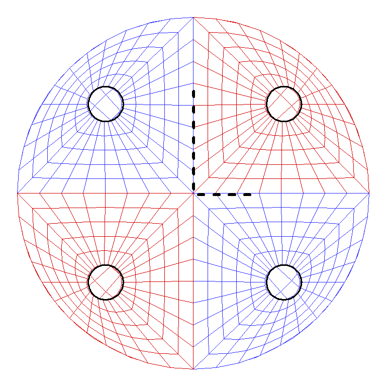
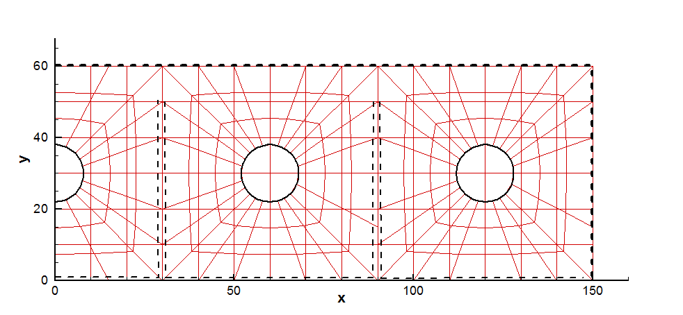
This procedure can be used with multiple waterlines, as in the case of a TLP, semi-sub, or catamaran. In these cases it is necessary to define quadrilateral partitions which separate the waterlines and serve to define the outer boundaries of local patches surrounding each waterline. Examples of these inputs are shown below for the TLP and semi-sub. When partitions are used for this purpose, certain restrictions must be followed:
- The patches defined by the partitions and the waterline of the outer control surface must cover the free surface with no gaps or overlaps.
- Each partition, as well as the outer waterline, must obey the rule that as one progresses in the positive direction from one vertex to the next, one passes around the waterline in a counter-clockwise direction as viewed from above the free surface.
- When multiple waterlines are defined by the GDF inputs, the order of the waterlines and the order of the partitions must correspond, with the same number of each. For example in TEST15 the columns of the semi-sub are defined starting at the midship section X=0 and moving out toward the bow, following the patch definitions of the subroutine SEMISUB in GEOMXACT; in this case the partitions in the CSF file must follow the same order, as shown in Example 4 below. A proper sequence of the patches and panels must be followed in the GDF file and geometry definition: all indices of the patches or panels belonging to each waterline must be either smaller or larger than all indices of the patches or panels belonging to the other waterlines. The order of these indices defines the order of the waterlines, and the partitions defined in the CSF file must follow the same order.
- When partitions are used to separate multiple waterlines the program will extend (or contract) the outer ends of the partitions so that they are located at the intersections with the outer boundary. Thus, as shown in Figures 11.1 and 11.2, it is not necessary for the user to compute the exact coordinates of the intersections. In these two Figures the coordinates of the intersections are obvious, but in some cases extra computation would be required, and the program is intended to perform this computation automatically. However in some cases the program may not identify end points which should be moved to the outer boundary, and the user should verify that this has been done correctly by plotting the data in the auxiliary file gdf_csf.dat. This problem can be avoided by specifying the correct vertex coordinates in the CSF file, for the outer ends of the partitions.
Automatic definition of the intermediate free surface may fail in some cases where the waterlines are irregular. Examples of ‘irregular’ waterlines where the automatic option may fail include: (1) locally concave waterlines, (2) moonpools, (3) bodies with thin elements (dipole patches) which intersect the free surface (e.g. TEST21), and (4) bodies with horizontal patches or panels in the plane of the free surface. It is advisable to confirm the representation of automatic control surfaces by plotting the data in the auxiliary file gdf_csf.dat. In cases where only the horizontal components of the drift force and vertical component of the drift moment are required, the intermediate free surface can be omitted.
The option to use two separate CSF files, described in Section 11.4 above, should not be used for automatic control surfaces.
When automatic representation of the control surface is used, special values must be assigned to the parameters NPATCSF and ICDEF, as defined below, and the complete CSF file should be of the following format:
1 (ILOWHICSF)
ISXCSF ISYCSF
NPATCSF ICDEF PSZCSF
RADIUS DEPTH
NPART
NV(1)
X(1,1) Y(1,1)
X(1,2) Y(1,2)
.
.
.
X(1,NV1) Y(1,NV1)
NV(2)
X(2,1) Y(2,1)
X(2,2) Y(2,2)
.
.
.
X(2,NV2) Y(2,NV2)
NV(NPART)
X(NPART,1) Y(NPART,1)
X(NPART,2) Y(NPART,2)
.
.
.
X(NPART,NV1) Y(NPART,NV1)
The symmetry indices ISXCSF and ISYCSF of the control surface must be the same as the symmetry indices ISX,ISY of the body. Here the body symmetry indices ISX,ISY are the same as the inputs in the GDF file, except in the case where the body is trimmed.
Special attention to symmetry is required if the body waterline is trimmed, since this may affect the symmetry of the body. If the trim includes a roll angle, XTRIM(3) is nonzero and ISY=0 regardless of the GDF input symmetry index. In this case ISYCSF=0 must be specified in the CSF file. Similarly, if the trim includes a pitch angle, XTRIM(2) is nonzero and ISXCSF=0 must be specified.
For cases where NBODY>1 and one or more bodies have planes of symmetry, as specified in the GDF file, and no trim angles are specified for the body, then the same planes of symmetry should be specified for the control surface (regardless of the fact that no symmetry is used for the potential solution). In this case the control surface is reflected in the same manner as the body. Tests 05 and 13 are examples of this convention.
If incorrect symmetry indices are input in the CSF file an error message is issued and the run is terminated.
NPATCSF must be equal to zero or less than zero:
NPATCSF=0: the control surface is automatic and includes the intermediate free surface
NPATCSF<0 the control surface is automatic and the intermediate free surface is omitted
ICDEF must be equal to zero:
ICDEF=0: the control surface is automatic
RADIUS is the parameter which controls the radius of a circular outer surface, or specifies that the outer surface is quadrilateral:
RADIUS>0: the outer surface is a circular cylinder of this radius
RADIUS≤0: the boundary of the outer surface is quadrilateral with NV(1) vertices specified by the coordinates (X(1,n), Y(1,n)) (n=1,2,...,NV(1)).
DEPTH is the depth of the control surface. This must be a positive real number, greater than the maximum depth (draft) of the body.
NPART is an integer which specifies the number of partition boundaries. Each partition boundary includes NV vertices, defined by the coordinates X,Y. Partition boundaries are required for two possible purposes, (a) to define the outer boundary of a quadrilateral control surface, and (b) to separate multiple waterlines. If the body has only one waterline and the outer boundary is circular, NPART=0. If the body has only one waterline and the outer boundary is a quadrilateral, NPART=1. When the outer boundary is a quadrilateral its vertices must be defined by the first partition, with NV(1) vertices, and other partition boundaries (if any) must be included after this in the file.
The vertex coordinates (X,Y) must be ordered so the partition boundaries enclose the waterlines in the ‘counter-clockwise’ direction, as illustrated in the examples below.
In cases where there are no planes of symmetry, each waterline is a closed curve which must be surrounded by a closed partition boundary. When there is more than one waterline the partition boundaries must not overlap, nor should gaps exist between them.
In cases where the body is symmetric about X=0 and/or Y=0, and the same symmetry planes are used for the CSF, the completeness of the partition boundaries depends on whether or not the waterline intersects the planes of symmetry. If the waterline is entirely within the interior of a quadrant or half-space and does not intersect the symmetry plane(s), then it must be completely enclosed by a partition boundary. If the waterline intersects a symmetry plane then the partition boundary should not include that plane, since it will be closed by reflection about the plane.
For patches on the free surface, the parametric coordinates are defined with U=+1 on the body waterline and U=-1 on the outer partition boundary; V is positive in the counter-clockwise direction around body waterline. When a circular cylindrical outer surface is used (IPARTR=1) U is in the azimuthal direction and V is in the vertical direction on the side and radial direction on the bottom.
Several examples of .csf files are included below to illustrate the use of partition boundaries. (Header lines are omitted for brevity.)
Example 1: single waterline with circular outer boundary, as in TEST01c and TEST13c:
1 ILOWHICSF
1 1 ISX ISY
0 0 1. NPATCSF ICDEF PSZCSF
1.2 2.2 RADIUS, DEPTH
0 NPART
Example 2: single waterline with quadrilateral outer boundary, as in TEST15 and TEST22:
1 ILOWHICSF
1 1 ISX ISY
0 0 0.5 NPATCSF ICDEF PSZCSF
0.0 0.3 RADIUS, DEPTH
1 NPART
3 NV(1)
2.2 0.0
2.2 0.3
0.0 0.3 (X,Y coordinates of three vertices)
Note in Example 2 the partition boundary is specified only in quadrant one, since ISX=1 and ISY=1. The first vertex is on the +x-axis, the second vertex is above the first, and the third vertex is on the +y-axis to close the partition and surround the body waterline. The order of the vertices is such that they follow a counter-clockwise progression around the body with increasing polar angle relative to a point inside the body.
Example 3: TLP or semi-sub with four columns and two planes of symmetry with a circular outer boundary, as in TEST06b and TEST14:
1 ILOWHICSF
1 1 ISX ISY
0 0 10. NPATCSF ICDEF PSZCSF
85.0 40.0 RADIUS, DEPTH
1 NPART
3 nv1
0.0 50.0
0.0 0.0
30.0 0.0 (X,Y coordinates of vertices)
In this case, since the waterline is a closed curve in the interior of quadrant one, the partition boundary is required to separate the waterline in quadrant one from the other three waterlines of the TLP. The partition boundary is down, along the +y-axis, and then to the right along the +x-axis, in accordance with the ‘counter-clockwise rule’. This example illustrates a useful feature that the outermost points do not need to intersect the outer boundary; the program extends or reduces the first and last segments automatically, to intersect the outer boundary (the inputs 50.0 and 30.0 could be replaced by any positive numbers).
Example 4: ten waterlines, two and a half in each quadrant, with rectangular outer boundary, as in TEST15 (semi-sub with a total of ten columns):
1 ILOWHICSF
1 1 ISX ISY
0 0 10. NPATCSF ICDEF PSZCSF
0.0 40.0 RADIUS, DEPTH
4 NPART
3 NV(1)
150.0 0.0
150.0 60.0
0.0 60.0 end of partition 1 (outer boundary of control surface)
3 NV(2)
0.0 0.0
30.0 0.0
30.0 50.0 end of partition 2 (encloses middle half-column)
4 NV(3)
30.0 50.0
30.0 0.0
90.0 0.0
90.0 50.0 end of partition 3 (encloses second column)
3 NV(4)
90.0 50.0
90.0 0.0
150.0 0.0 end of partition 4 (encloses third column)
In this case the first partition boundary defines the outer rectangular boundary of the control surface, and the other three are required to separate the waterlines in quadrant one. Note that partition 2 starts at the origin in this case, without a segment along the y-axis, since only half of the middle column is in the first quadrant and the images of both the body and partition form a closed waterline and partition. As in Example 3 the outermost points do not need to intersect the outer boundary; the program extends or reduces the first and last segments automatically, to intersect the outer boundary (the inputs 50.0 are replaced by 60.0). For the last vertex (150, 0) the X-coordinate could be replaced by any value greater than 90.0. All four partitions obey the ‘counter-clockwise rule’ with respect to their domains. Also note that they completely define the interior free surface, without gaps or overlap. In this example, if only the horizontal drift forces and vertical drift moment were required, one could assign NPATCSF=-1 and NPART=1, and omit all but the first partition.
The view of this control surface from above the free surface is shown in Figure 11.2.
Example 5: Monohull with one plane of symmetry, as in TEST22 (FPSO with internal tanks) using a rectangular outer control surface:
1 ILOWHICSF
0 1 ISX ISY
0 0 2. NPATCSF ICDEF PSZCSF (1st two indicate this is automatic)
1 NPART
4 nv0
12.0 0.0
12.0 3.0
-12.0 3.0
-12.0 0.0
In this case the outer rectangular boundary has four vertices, starting on the +x axis and ending on the -x axis.
When automatic representation of the CSF is implemented, the program traces the body waterline(s) and establishes extra patches or panels on the free surface between these waterlines and the partition boundaries. When the program connects adjacent sides of patches in the waterline, the patches or panels are identified based on the coincidence or close proximity of their vertices. The parameter TOLGAPWL is used for this purpose, to allow for small gaps (or overlaps) between adjacent patches at the waterline. The default value TOLGAPWL=10-3 is used unless a different value of this parameter is defined in the CFG file, as explained in Section 4.7. In the test for adjacent patches the nondimensional Cartesian coordinates of the adjacent patch corners are evaluated, and the distance between these points is computed. The patches are assumed to be connected if this distance is less than either TOLGAPWL or the product of TOLGAPWL and the maximum length of one of the patch sides. The latter value is introduced to allow for cases where the size of the structure is much larger than the characteristic length ULEN. The default value is recommended in general. If the program is unable to close a waterline using this value, an error message is displayed stating that the waterline is not closed. The default value is recommended in general. If the program is unable to close a waterline using this value, an error message is displayed stating that the waterline is not closed. In that case a larger value of TOLGAPWL should be input in the CFG file.
The automatic CSF option should not be used for a body which is totally submerged. This case can be handled more simply, by using one of the GEOMXACT subroutines which represent closed bodies with an additional patch on the interior free surface, as one would do to remove irregular frequencies (IRR=1). This option is included in the GEOMXACT subroutines CIRCCYL, ELLIPCYL, SPHERE, ELLIPSOID, or BARGE, as explained in Section 7.8. Alternatively, one can use ICDEF=0 as explained above in Section 11.3, and include one or more quadrilateral patches to represent the interior free surface.
11.6 OUTPUT
The mean forces and moments using a control surface are output in the OUT file and in the numeric output file optn.7 or frc.7 in the same format as used for pressure integration (Option 9).
When IPLTDAT> 0 in the CFG file, the auxiliary file gdf_csf.dat is output. This can be used for visualization of the control surface, using TecPlot or other similar programs. As in the case of the corresponding data files for visualizing the body surface the data in this file are defined with respect to the global coordinate system, and when NBODY>1 there is only one output file with the filename associated to the first body.
When ILOWHICSF= 1 and ILOWGDF> 0 in the CFG file, the file gdf_low.csf is output. This contains the data of the control surface in the low-order form described in Section 11.2.
TEST05, TEST13 and TEST22 show examples of using the control surface in the evaluation of the mean forces and moments.