
Chapter 12
SPECIAL EXTENSIONS
12.1 INTERNAL TANKS
WAMIT includes options to analyze the linear hydrodynamic parameters for a fluid inside an oscillatory tank, or to analyze the coupled problem where one or more tanks are placed within the interior of one or more bodies, including their dynamic coupling. Usually the fluid in each tank is bounded above by a free surface, but in special cases a rigid boundary surface can be placed above the fluid to represent a tank entirely filled by fluid.
In special cases where the tank is entirely filled and bounded above by a rigid surface the solution for the velocity potential is non-unique, and an arbitrary constant can be added to the potential or pressure without affecting the boundary conditions. Usually it is possible to obtain appropriate solutions for hydrodynamic outputs such as the added-mass coefficients, which are not affected by the non-unique constant, but the results of such computations should be checked to ensure that they are physically reasonable, and not affected by adding a constant to the potential or pressure.
The following discussion pertains to the situation where a free surface is present in each tank. The free surface boundary condition in each tank is linearized in the same manner as for the exterior free surface. Special attention is required near the eigenfrequencies of the tanks, where nonlinear effects are significant. The method described in Section 12.8 can be used to damp resonant tank motions, as illustrated in TEST07 and TEST22.
The tank geometry is defined in the same manner as for the exterior surface of each body, using either the low-order or higher-order method. In both cases it is essential that the normal vector points away from the ‘wet’ side of the tank surface, as explained in Section 6.1 (ILOWHI=0) and Section 7.1 (ILOWHI=1). In the context of a tank, this means that the positive normal vector points out of the tank and into the space exterior to the tank. In the low-order method the tank panels are included with the conventional body panels in the .GDF file. In the higher-order method the tank patches are defined in the same manner as the body surface, using one of the options listed in Sections 7.5-7.9. In both cases the tank panels or patches are identified by their starting and ending indices, which must be listed in the configuration files using the parameter NPTANK as explained in Section 4.7.
TEST07 and TEST22 are examples, where the body is an FPSO containing two rectangular internal tanks. In TEST07 panels 1-308 represent the exterior surface of the hull and the remaining panels represent the tanks. In TEST22 patches 1-7 represent the exterior surface, patches 8-11 represent tank 1, and patches 12-15 represent tank 2. (When IRR=1, this convention is modified, with patches 8-10 used for the interior free surface of the FPSO and patches 11-18 used for the tanks, as explained in the header of the GEOMXACT.DLL subroutine FPSOINT.) One side of each tank is represented by four rectangular patches, with their vertex coordinates included in the GDF file test22.gdf.
The panels or patches which represent each tank must be contiguous. Separate tanks can be grouped together, or interspersed arbitrarily within the description of the exterior surface. It is recommended to group all of the tanks together, either at the beginning or at the end of the panels/patches which define the exterior surface.
The vertical positions of tanks can be specified arbitrarily, and the free surface of each tank can be defined independently of the other tanks and the exterior free surface. Two alternative options can be used to specify the elevations of the tank free surfaces, depending on the parameters ZTANKFS and ITRIMWL in the CFG file.
If ITRIMWL=0, or if ZTANKFS is not included in the CFG file, then for each tank the free surface is defined to coincide with the highest point of the panel vertices or patch corners defining that tank. This option is illustrated in TEST 22, where the free surface of one tank coincides with the exterior free surface, i.e. the plane Z = 0, and the free surface of the other tank is elevated by 1m above this plane.
If ITRIMWL≥1, and the array ZTANKFS is included in the CFG file, the free surface of each tank is defined to be at the elevation above Z = 0 specified by the corresponding element of ZTANKFS. This option can be used to vary the filling ratio of tanks, without changing the GDF inputs, and also to trim the waterlines of the tanks so that the free surfaces remain level when the vessel is trimmed. Further information is given in Section 12.2. This option is illustrated in TEST22a, where the vessel is given a heel (static roll) angle of 15 degrees, and also in TEST22b where the tanks are partially filled. When this option is used, the geometry of the internal tank surfaces must be defined up to (or above) the trimmed free surface of the tank.
Special attention is necessary if the origin of the body coordinate system is above or below the plane Z = 0 of the exterior free surface (XBODY(3,K) is nonzero in the Potential Control File as defined in Section 4.2). If ITRIMWL=0, or if ZTANKFS is not included in the CFG file, and ZTANKFS is assigned by the program from highest point of the panel vertices or patch corners defining that tank, the value is assigned in body coordinates. However if ZTANKFS is assigned in the CFG file, it must be defined there in global coordinates to correspond with the elevation above the exterior free surface. In all cases, when tanks are included, the values of ZTANKFS shown in the Tank parameters list in the header of the .out file are defined in body coordinates, to be consistent with the hydrostatic parameters of the tanks. These details are illustrated in TEST22b.
The solutions for the velocity potential (or source strength) are performed independently for the exterior fluid domain, and for each interior tank. Thus the mutual locations of these surfaces are irrelevant. Small gaps between them do not cause problems, and they may even coincide without introducing numerical difficulties. When irregular-frequency removal is used (IRR>0), the entire interior free surface inside the body should be described, ignoring any possible intersections with tanks. Thus the same interior free surface should be used with or without the presence of tanks.
Two types of tank parameters must be included in the CFG file, as explained in Section 4.7:
NPTANK is an integer array used to specify the panel or patch indices of internal tanks. The data in this array are in pairs, denoting the first and last index for each tank. An even number of indices must be included on each line, and each pair must be enclosed in parenthesis. More than one line can be used for multiple tanks, and/or multiple tanks can be defined on the same line. If NBODY>1, the body numbers for each body containing tanks must be appended to the parameter name. Only integer data and parenthesis are read for the array NPTANK. Other ASCII characters may be included on these lines, and are ignored when the input data is read.
RHOTANK is a real array used to specify the density of fluid in internal tanks. The density specified is relative to the density ρ of the fluid in the external domain outside the bodies, as defined in Chapter 3 and Section 4.4. The data in the array RHOTANK must be input in the same order as the data in the array NPTANK. Multiple lines of this parameter may be used, with an arbitrary number of data on each line, but each line must begin with ‘RHOTANK=’. The total number of tanks NTANKS is derived from the inputs NPTANK in the POTEN run. If fewer than NTANKS values of RHOTANK are specified, the remainder of the array is assigned the last non-negative value. Thus if the density is the same for all tanks, only the first value is required. Zero may be assigned, but negative values of the density must not be assigned. RHOTANK is only used in the FORCE run, and may be changed if separate FORCE runs are made using the same POTEN outputs.
The following are equivalent formats for the required lines in the file test22.cfg:
NPTANK= (8-11) (12-15) (patch/panel indices for two tanks)
RHOTANK= 0.6 0.6 (fluid densities for tanks one and two)
NPTANK= (8 11) (patch/panel indices for tank one)
NPTANK= (12 15) (patch/panel indices for tank two)
RHOTANK= 0.6
These examples illustrate the following rules:
- Only integer data are recognized in NPTANK. Arbitrary ASCII characters other than these can be used both as comments and to delimit the pairs of indices for each tank, according to the user’s preferences. At least one blank space must be used to separate pairs of indices. Comments appended to these lines must not include integer characters.
- The total number NTANKS of tanks to be included is determined by the number of pairs of indices in NPTANK inputs, in this case NTANKS=2. The same number of densities RHOTANK is required for the analysis, but it is not necessary to input repeated values if all of the densities are the same (or if all of the densities after a certain point are the same). The order of the tank densities must correspond to the order of the index pairs in NPTANK.
- The data in RHOTANK are real numbers. After specifying all NTANKS values, arbitrary comments can be appended as in the first example above, but if fewer than RHOTANK real numbers are assigned the remainder of the line should be left blank, as in the second example above.
The real array ZTANKFS can be included in the configuration files, as explained in Section 4.7, to specify the free-surface elevations in internal tanks. The data in this array define the elevations of the tank free surfaces, above the plane Z= 0 of the exterior free surface. The data in the array ZTANKFS must be input in the same order as the data in the array NPTANK. Multiple lines of this parameter may be used, with an arbitrary number of data on each line, but each line must begin with ‘ZTANKFS=’. If the array ZTANKFS is included, it must include one real number for each tank. If the array ZTANKFS is not included, the waterline of each tank is derived from the highest vertex of the GDF inputs. ZTANKFS is only used when the waterline trimming parameter ITRIMWL≥1, as explained in Section 12.2. The data in ZTANKFS are dimensional, with the same units of length as are used in the GDF file.
Special inputs are required when pressures and/or velocities are evaluated for field points inside the tanks (Option 6). In this case, when the field point coordinates XFIELD are input as explained in Section 4.3, the parameter ITANKFPT=1 must be specified in the .cfg file, as explained in Section 4.7, and the format of the XFIELD inputs in the .frc file must include the corresponding number of each tank, or zero for the exterior domain. When all of the field points are defined by arrays, using the option described in Section 4.11, the parameter ITANKFPT is not used and may be deleted from the .cfg file.
When IOPTN(6) is nonzero the output pressure and fluid velocity are computed for the specified points fixed in space, as in the case of the same outputs in the exterior domain. To evaluate the corresponding values following these points when they are fixed relative to the tanks on a moving body, changes due to the body motion should be added as in (15.63).
Inputs which relate to the body’s mass including VCG and the radii of gyration XPRDCT (IALTFRC=1), or XCG, YCG, ZCG and the inertia matrix EXMASS (IALTFRC=2) refer to the mass of the body alone, without the tanks (or with the tanks empty). The same definitions apply to the outputs of these quantities in the .mmx file described in Section 5.6, and in the log file wamitlog.txt. When IALTFRC=1 is used, the body mass is derived from the displaced fluid mass corresponding to the body volume, minus the fluid mass in the tanks.
The body volumes, center of buoyancy, and hydrostatic restoring coefficients displayed in the header of the .out file are calculated from the exterior wetted surface of the body, and are not affected by the tanks. The volumes, densities, values of ZTANKFS, and hydrostatic restoring coefficients for the tanks are listed separately after the corresponding data for the hull. When the higher-order option (ILOWHI=1) is used, the header of the .out file includes a list of all the patches, and the corresponding tank numbers ITANK for patches which are defined as interior tanks. When ITRIMWL=0 or ZTANKFS is not included in the CFG file, the values of ZTANKFS displayed in the header of the .out file correspond to the tank free-surface elevations as used in the program, derived from the upper boundary of the tank surfaces.
Hydrodynamic parameters which are physically relevant for the tanks alone (Options 1,5,6,9) can be computed by inputting only the patches or panels for the tanks. In this case IDIFF=-1 should be used, and the outputs for options 5,6,9 correspond to the combination of radiation modes specified by the IMODE array, with unit amplitude of each mode. The damping coefficients for the tanks should be practically zero. From momentum conservation the horizontal drift forces and vertical drift moment from Option 9 should be practically zero.
Internal tanks affect the hydrostatic restoring coefficients Cij, as described in Section 15.10. The hydrostatic matrix, which is output in the out and hst files, includes the effects of the tanks. For example the hydrostatic coefficient C33 in the output files is equal to the total area of the waterplane inside the waterline of the body, minus the product of the free-surface area and density for each tank. When both tanks and the external hull surfaces are included, hydrodynamic and hydrostatic parameters which are relevant for the hull alone, with no internal tanks, can be computed by setting RHOTANK=0.0
When planes of symmetry are specified in the GDF file (ISX=1 and/or ISY=1) the tank geometry is reflected in the same manner as the hull. This procedure should only be used if all of the tanks intersect the symmetry plane (with half of the tank on each side of the plane). For example in the case of the FPSO shown in Appendix A.22, where both tanks extend across the plane of symmetry Y=0, it is appropriate to use ISY=1 as is done in TEST22. On the other hand if there are separate tanks on each side of the symmetry plane (e.g. wing tanks) the hydrostatic and hydrodynamic coefficients for the tanks will not be physically correct. This situation can be avoided by defining both sides of the hull and both tanks separately in the GDF file, and setting ISY=0.
12.2 TRIMMED WATERLINES
WAMIT includes the option to specify a ‘trimmed waterline’ for each body. In the trimmed condition, the static orientation of the body is shifted relative to the horizontal plane of the free surface, first by a prescribed vertical elevation, then by a pitch angle (often referred to as the ‘trim angle’), and then by a roll angle (‘heel’). For a given body geometry, different planes of flotation can be analyzed without redefining the geometry in the GDF file. A necessary condition for this procedure to be implemented is that the definition of the body geometry in the GDF file must include all surface elements which are submerged when the body is trimmed. Thus it is necessary to define a sufficient portion of the body surface above the untrimmed waterplane.
Trimming of the waterline is supported in both the low-order (ILOWHI=0) and higher-order (ILOWHI=1) methods. There are some practical restrictions that must be considered when the higher-order option is used, as described below.
The trimmed condition of the body is specified by two parameters in the configuration files, ITRIMWL and XTRIM, as defined in Section 4.7. ITRIMWL=0 is the default, indicating that the body is not trimmed. ITRIMWL≥1 specifies that the body is trimmed, and XTRIM(1:3) specifies the vertical elevation and angles of rotation of the body, as explained below. If ITRIMWL=0, XTRIM is ignored. Note that if ITRIMWL=0 (or ITRIMWL is not included in the inputs), then the GDF file must only define the submerged portion of the body as in previous versions of WAMIT; in this case the program checks to ensure that no elements of the body surface are above the plane of the free surface, and an error stop occurs if such elements are detected. Conversely, when ITRIMWL≥1, elements of the body surface above Z=0 are permitted, and there is no check or error stop. It is possible to suppress the error stop, without trimming, with the inputs ITRIMWL=1 and (XTRIM=0.0 0.0 0.0).
Special attention is required when the submerged surface is changed by trimming to ensure that it intersects the free surface in one or more closed waterlines. If any points on the original waterline are moved vertically downward by the trimming it is necessary to define a sufficiently high portion of the original surface, above the untrimmed waterline, in the GDF file. There is no error check in the program to check that the trimmed surface is in contact with the free surface, and small gaps may be difficult to see if the trimmed surface is visualized. It is important to check that the three volumes (VOLX,VOLY,VOLZ) in the header of the .out output file are equal, with a small tolerance for differences that is comparable to the differences in the untrimmed state.
ITRIMWL=1 is the usual option when trimming is specified. In the higher-order method (ILOWHI=1) it may be necessary to assign a larger value of ITRIMWL to correctly identify the trimmed waterline in cases where it intersects one side of a patch at more than one point. An example of this situation is shown in TEST22a, where ITRIMWL=2 is required. This cannot occur in the low-order method (ILOWHI=0), since the sides of low-order panels are straight lines. If (ILOWHI=0) and ITRIMWL>1 the result is the same as ITRIMWL=1.
Appendix A includes four test runs with trimmed waterlines: TEST01A, TEST09A, TEST13A, and TEST22A. The perspective plots which accompany these descriptions illustrate the trimmed conditions of the structures.
When multiple bodies are analyzed, the vector XTRIM must be input separately for each body, following the same format as for XBODY in Section 8.4. TEST13A illustrates this procedure for NBODY=2.
The following coordinate systems and input parameters should be considered in defining the process of trimming waterlines:
(X,Y,Z) are global coordinates with Z=0 in the plane of the free surface.
(x,y,z) are conventional body coordinates, which define the submerged body surface in WAMIT.
(ξ,η,ζ), referred to hereafter as ‘GDF coordinates’, are the coordinates used to define the body geometry in the GDF file.
In the low-order method (ILOWHI=0), when the panel vertices are input from the GDF file, these are converted from GDF coordinates to body coordinates, using the translation and rotations defined by XTRIM. When the higher-order method is used (ILOWHI=1), the same coordinate transformations are performed from the subroutine outputs each time that the subroutine defining the body surface is called. The practical effect, in both cases, is that the original definition of the body geometry in the GDF file is replaced during the WAMIT computations by a new transformed description in (x,y,z) coordinates, which represents only the submerged portion of the body in the trimmed condition. This submerged surface can be plotted and visualized, in the same manner as for untrimmed bodies, using the parameter IPLTDAT as explained in Section 4.7.
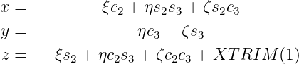
The transformation from GDF coordinates to body coordinates is defined by the following relations:
The perspective figures in the Appendix Section A.2 are useful to illustrate this transformation. The original GDF coordinates for the body are as shown in the first figures for TEST22, with the vessel in its conventional orientation. The GDF inputs for TEST22a are the same, except that the draft and tank depths are increased, so that after vertical trimming and applying the roll angle the entire surface is still submerged. After trimming the vessel is as shown in the perspective figures for TEST22a, which correspond to the new body coordinates with the z-axis vertically upward. The WAMIT outputs which result from TEST22a are the same as if the original GDF data defined the configuration shown in the TEST22a perspective figures, without trimming, and with the hull and tank waterlines as shown in these figures. The geometric output files (test22a_pat.dat, test22a_pan.dat, test22a_low.gdf) all correspond to the latter figures, not to the original un-trimmed GDF data. It is recommended to plot and visualize the geometry after trimming, using the data files which are defined by the parameter IPLTDAT in the CFG file, to ensure that the actual trimmed structure is correct.
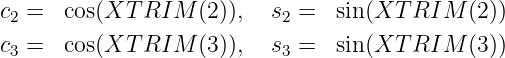
Except for the GDF coordinates, the definitions of coordinate systems, etc., are as defined in earlier chapters. In particular, the body motions and forces are defined with respect to the conventional body coordinates (x,y,z). Thus, for example, surge is in the horizontal direction and heave is in the vertical direction, relative to the free surface. Rotations and moments are defined with respect to the origin of this coordinate system. XBODY(1), XBODY(2), XBODY(3) are the (X,Y,Z) coordinates of the origin of the body coordinate system relative to the global coordinate system, and XBODY(4) is the angle in degrees of the x-axis relative to the X-axis of the global system in the counterclockwise sense, as shown in Figure 6.2.
The mass and inertia parameters in the FRC file are defined with respect to the body coordinates, and apply to the trimmed configuration as if it was the original input for the run. The outputs in the MMX file can be checked to verify that these are correct in the body coordinate system.
The input parameter XTRIM(1), which defines the vertical coordinate z of the origin of the GDF coordinates, is in the same units as the dimensional GDF coordinates, corresponding to the parameter GRAV in the GDF file. The angles XTRIM(2) (pitch) and XTRIM(3) (roll) are in degrees. XTRIM(2:3) are Euler angles, with the convention that the body is first pitched about the transverse η-axis, and then rolled about the longitudinal ξ-axis. (Yaw can be included via XBODY(4). With this convention the projection of the ξ-axis on the plane Z=0 is at the same angle XBODY(4) as the projection of the x-axis.)
In the low-order method (ILOWHI=0), the input panels from the GDF file are tested for their positions relative to the plane of the free surface (Z=0). ‘Dry’ panels, which are entirely above the free surface, are removed from the array of panel coordinates within the program. ‘Wet’ panels, which are entirely submerged, are retained without modification. Panels which intersect the waterline, referred to as ‘waterline panels’, are trimmed at the waterline. In some cases, where waterline panels have three vertices below the free surface and one vertex above the free surface, the resulting trimmed panel is a polygon with five sides; in these cases the panel is subdivided to form two separate panels (one quadrilateral and one triangular). The number of panels is increased by one for each subdivided panel. Conversely, when dry panels are removed, the number of panels is decreased. Examples of subdivided panels can be seen in the perspective plot corresponding to TEST01A in Appendix A.
In the higher-order method (ILOWHI=1), an analogous procedure is followed for each patch of the body, based on the vertical positions of the four corners of each patch. If the patch intersects the waterline, an iterative procedure is used to remap the submerged portion onto a square domain in parametric space. There are situations where this procedure breaks down, and thus it must be used with caution. One example is where the vertices of a patch are all submerged, but a portion of one side maps in physical space above the free surface. In that case it is necessary to assign ITRIMWL>1 as explained above. If ITRIMWL>1 the side is sub-divided into ITRIMWL segments and the search for the waterline intersection points is based on the elevation of the end-points of each segment.
Body symmetry can be affected by trimming. When it is necessary, WAMIT automatically reflects the body geometry and resets the symmetry indices. For example in TEST01A the GDF file specifies ISX=ISY=1, but the trimmed body has only one plane of symmetry (x=0). Similarly in TEST22A the GDF file specifies ISY=1, but the trimmed body has no planes of symmetry due to the heel angle.
Dipole panels are trimmed in the same manner as conventional panels, as illustrated in TEST09A.
Special attention is required for bodies with internal tanks. Two alternative options are included, as explained in Section 12.1, depending on the parameter array ZTANKFS in the CFG file. If ZTANKFS is not included in the CFG file (or if ITRIMWL=0), the geometry of internal tanks is not trimmed, and the tank free surface is always defined by the highest points of the specified panels or patches. If trimming includes a pitch or roll displacement of the body, this approach requires the tank geometry to be redefined so that its upper boundary coincides with the correct plane of the free surface inside the tank. If ZTANKFS is included in the CFG file (and if ITRIMWL=1), the geometry of internal tanks is trimmed using the same algorithms as for the exterior surface. In this case it is necessary to define the tank geometry up to the level of the trimmed free surface, as in TEST22A.
Special attention is required also when irregular-frequency removal is used (IRR>0). If the interior free surface is defined by the user as part of the overall geometry of the body (IRR=1) it is necessary to ensure that the interior free surface coincides with the Z=0 plane after trimming. If automatic discretization of the interior free surface is used (IRR=3), the interior free surface is defined correctly in the plane of the trimmed free surface. The option (IRR=2) cannot be used when ITRIMWL>0 (See Section 10.2).
12.3 RADIATED WAVES FROM WAVEMAKERS IN TANK WALLS
Different options are available for the analysis of problems where walls are present in the plane(s) of symmetry x = 0 and/or y = 0. The analysis of wave radiation by wavemakers in the plane(s) of the walls is discussed in this Section. A more general approach applicable to wavemakers in the planes of the walls and/or bodies in the interior domain of the fluid is described in Section 12.4. These two approaches require somewhat different inputs.
Either one tank wall of infinite width, or two semi-infinite walls at right angles, can be considered. These correspond to one or both of the symmetry planes x = 0 and/or y = 0. Wavemakers with prescribed normal velocities are located in the walls. The opposite walls of the wave tank are assumed to have absorbing beaches, represented here by open domains extending to infinity. In all cases it is assumed that the wall(s) are planes of symmetry, and the fluid motion is symmetrical about these planes. Thus the solution for the velocity potential in the fluid domain can be represented by a distribution of sources of known strength, proportional to the normal velocity of the wavemaker, and it is not necessary to solve the integral equation for the velocity potential on the wavemakers. This saves considerable computational time, and also avoids the singular solution that would otherwise occur for bodies of zero thickness in the plane of symmetry.
The geometry of each wavemaker is defined in the .gdf file. In the low-order method (ILOWHI=0) a sufficient number of panels must be included on each wavemaker to ensure a converged solution. In the higher-order method (ILOWHI=1) only one patch is required on each wavemaker. If the wavemakers are rectangular (or quadrilateral), the higher-order analysis can be carried out most easily using the option IGDEF=0, as explained in Section 7.5.
The parameter ISOLVE=-1 is used in the configuration files to indicate that the wavemakers are in planes of symmetry, and that the solution of the integral equation is not required. Suitable generalized modes must be defined, as explained in Chapter 9, to represent the normal velocity of each wavemaker. IRAD=0 is recommended, with IMODE(1:6)=0, to avoid computing the 6 rigid-body modes. IDIFF=-1 is required. The separate wavemaker elements are considered to be part of one ‘body’, with appropriate generalized modes used to represent the independent motion of each element, and NBODY=1. No other bodies can be present within the fluid domain.
The principal outputs are the potential and fluid velocity at specified field points (Option 6). If the field point is on the free surface the potential is equivalent to the wave elevation, as explained in Chapter 3. No other Options in the FRC file are supported. If multiple wavemakers are run together with separate modes for each wavemaker, the parameter INUMOPT6=1 should be specified in the .cfg file to provide separate outputs for each mode. In that case only the complex amplitude is output, with a separate pair of columns for each mode, as indicated in Section 5.2. A post-processor should be used to combine these outputs, for arbitrary combinations of simultaneous motion of all wavemakers.
The subroutine WAVEMAKER is included in the NEWMODES DLL file, to analyze one or more wavemakers. If IGENMDS=21 is specified in the configuration files the wavemakers are hinged with pitching motions about a horizontal axis. The depth of this axis is specified in the input file gdf_wmkrhinge.dat where gdf is the filename of the GDF file. In the subroutine the depth of the axis is the same for all wavemaker elements. The number of wavemakers is arbitrary, but each separate mode of motion corresponds to one patch (or panel) of the geometry, in the same order as these are defined in the .gdf file. In the low-order method this effectively restricts the use of the subroutine to only one panel per wavemaker. Thus it is strongly recommended to use the higher-order method (ILOWHI=1) when using the subroutine WAVEMAKER. NEWMDS=NPATCH must be specified in the pot or cfg file, with the same value as the number of patches in the gdf file.
The subroutine WAVEMAKER includes two additional options, specified by IGENMDS=211 and IGENMDS=212. If IGENMDS=211 each wavemaker is like a piston, with constant normal velocity on its surface. If IGENMDS=212 a bank of contiguous wavemakers are joined by vertical hinges, and represented by tent functions with constant normal velocity in the vertical direction. Further information is given in the header of this subroutine.
TEST23, described in Appendix A.23, illustrates the use of the option IGENMDS=21 for a bank of eight wavemakers along the wall x = 0, with symmetry about both x = 0 and y = 0. The generated wave elevations for each wavemaker are evaluated over a square array of 8 × 8 = 64 field points. The depth of the horizontal axis is specified by the parameter ZHINGE=-2m in the input file test23_wmkrhinge.dat.
12.4 BODIES AND WAVEMAKERS WITH VERTICAL WALLS
WAMIT includes the option to account for images of the body in the presence of one vertical wall, or two vertical walls which intersect at a right angle. The presence of walls is specified by the optional integer inputs IWALLX0 and IWALLY0 in the configuration files. In the default case these inputs are assigned the values zero, signifying that there are no walls. The inputs IWALLX0=1 and/or IWALLY0=1 signify that there are walls in the planes x = 0 and/or y = 0, respectively. All other inputs are unchanged from the case without walls. In particular the GDF files for one or more bodies should specify the symmetry indices ISX,ISY corresponding to the planes of symmetry of the body, with values 0 or 1, just as in the case without walls.
Figure 12-1 defines two coordinate systems, one fixed on the body and the other on the wall. The axes of the former are denoted by (x,y,z) and those of the latter by (X,Y,Z). In the presence of wall(s), the global coordinate system defined in Section 4.2 must coincide with the wall coordinate system as defined in Figure 12.1.
In the Potential Control File the vector XBODY(1),XBODY(2),XBODY(3) specifies the dimensional (X,Y,Z) coordinates of the origin of the body-fixed coordinate system relative to wall system, in the units of the length ULEN. XBODY(4) is the angle in degrees formed by the body x-axis and the X-axis of the wall system, as defined in Figure 12.1. The values of the incident wave heading angles BETA are defined with respect to the positive X-axis.
An important detail to note is the definition of the incident-wave amplitude and its physical interpretation. The ‘incident-wave’ is defined as the incoming wave component prior to reflection from the wall(s), and A is the corresponding amplitude. If only one wall is present then, after reflection, the resulting wave field in the absence of the body is an oblique standing wave with maximum free-surface elevation 2A. In the special case β = 0 the incident wave propagates parallel to the wall, without a distinct reflected component, but the physical amplitude of this wave is 2A. Some consequences of this definition are noted in the comparison of Test Runs 04 and 19 (see Sections A.4 and A.19). If two walls are present, the resulting wave motion after reflection from both walls will have a maximum elevation of 4A.
In the Force Control File the array IOPTN is unchanged from the definitions in Section 4.3. Since momentum integration cannot be used to determine the mean drift force and moment, IOPTN(8)=1 is ignored. IOPTN(9) is used in the normal manner to evaluate the drift force and moment from pressure integration. IOPTN(7) can be used provided the control surface is within the fluid domain. The Haskind wave heading angles BETAH are defined with respect to the walls in the same manner as BETA. The coordinates of field points XFIELD where the pressure, wave elevation, and velocity are evaluated, are defined as in Section 4.3 relative to the wall-mounted system.
The incident-wave velocity potential is defined relative to the wall-mounted coordinate system. Consequently, the phases of the exciting forces, motions, hydrodynamic pressure and field velocity induced by the incident wave are understood relative to the incident-wave elevation at X = Y = 0. In addition the fluid velocity vector components are given with respect to the wall-mounted coordinate system.
The other definitions of output quantities in Chapter 3 are unchanged.
Wavemakers may be included in the walls, following a similar procedure as described in Section 12.3. When bodies and wavemakers are both present, ISOLVE≥0 must be specified. The wavemakers are treated as one or more separate bodies. In the simplest case, where one body is in the fluid domain and all wavemakers are defined within another GDF file, NBODY=2 is used and the parameter IBODYW=2 is defined in the CFG file, indicating that body 2 consists of wavemakers in the walls. The order of the bodies is specified by the order of the corresponding inputs in the POT file. There can be one or more physical bodies, and one or more wavemaker bodies. The physical bodies must precede the wavemaker bodies in all cases. Thus if K=1,2,...,NBDYP are the indices for NBDYP physical bodies, and K=NBDYP+1,NBDYP+2,...,NBDYP+NBDYW are the indices for NBDYW wavemakers, NBODY=NBDYP+NBDYW is the total number of bodies identified in the input files and IBODYW=NBDYP+1 is the index of the first wavemaker body, input in the configuration files.
Only the radiation problems are solved when wavemakers are present, including radiation from the wavemakers as generalized modes. Outputs with wavemakers include the added mass and damping matrices (Option 1), a surrogate for the Haskind exciting force to be explained below (Option 2), RAO’s in response to the Option 2 exciting force and moment (Option 4), as well as Options 5,6,7.
The ‘surrogate’ exciting force is the force and moment acting on the body due to the motions of the wavemakers, computed from the cross-coupling added mass and damping coefficients where one mode is for the body and the other mode is for the wavemaker. The outputs for the exciting force (Option 2) and RAO (Option 4) are the same as for incident waves, except that the index of the wavemaker is output in place of the wave incidence angle BETA. These ‘wavemaker RAO’s’ cannot be compared directly with the conventional incident-wave RAO’s since the amplitude of the waves generated by the wavemaker modes are not used to normalize the RAO’s. It is possible to make a separate run without the bodies to measure the wave elevations at the locations of the bodies using Option 6, as one might do to calibrate the wavemakers in a physical wavetank. If the wavemaker RAO’s are normalized by these calculations of the wave elevations the results are directly comparable with the conventional RAO’s in incident waves of unit amplitude.
When walls are specified by the parameters IWALLX0=1 and/or IWALLY0=1, the program automatically reflects the body and wavemaker geometry about the walls. The planes of symmetry for each body or wavemaker, defined by the parameters ISX and ISY in the GDF file, refer specifically to the local planes of symmetry of the body or wavemaker. When IWALLX0=1 and wavemakers are defined in the wall X=0, the symmetry index ISX=0 should be used for the wavemakers; similarly, for wavemakers in the wall Y=0, ISY=0. (Except for special cases where the GDF file only defines one half of the wavemaker, both wavemaker symmetry indices should be zero.) The symmetry indices for bodies are the same as without walls.
Since the wavemakers correspond to one or more bodies, it is necessary to include the usual inputs for these bodies in one or more FRC files. However, the dynamic characteristics of the wavemakers are ignored, since the RAO’s are not evaluated for the wavemakers. Thus dummy values of the inputs for the dynamic characteristics of the wavemakers (VCG and XPRDCT, or XCT and external force matrics) must be included, but their values are not relevant.
12.5 BODIES WITH PRESSURE SURFACES
Starting in Version 7.0 it is possible to analyze problems where part of the body surface consists of one or more free surfaces, on which the pressure distribution is specified instead of the normal velocity. These are referred to as ‘free-surface pressure’ surfaces (FSP). Practical examples of bodies with FSP surfaces include oscillating water columns used for wave-energy conversion and air-cushion vehicles which are supported by positive mean pressure acting on the free surface below the body.
FSP surfaces can be either in the same plane (Z = 0) as the exterior free surface, or submerged (Z < 0) below the level of the exterior free surface (corresponding to a positive static pressure imposed on the surface as in the case of an air-cushion vessel). All FSP surfaces must be in horizontal planes, corresponding to constant values of the static pressure on each surface. The theory for this extension is described in Section 15.11. Test 25 is an example of the use of this option.
The geometric definition of FSP surfaces is the same as for the other parts of the body surface, defined within the same GDF input file(s). The panels or patches which represent FSP surfaces are specified using the parameter NPFSP in the configuration files to identify the panel or patch indices. The inputs NPFSP must be in pairs, denoting the first and last values of the index (See Section 4.7). Multiple lines containing NPFSP=(N1 N2) can be used to indicate all of the FSP panels or patches for the body.
The oscillatory pressure distributions acting on the FSP surfaces are defined in a manner similar to the representation of generalized modes, using subroutines in the file newmodes.dll, as described in Chapter 9. In the simplest case the pressure distribution is constant, and only one mode is required for each FSP surface. In more general cases the pressure distribution can be represented by appropriate sets of modes such as Fourier modes. The parameters IMODESFSP and NMODESFSP specify for each body the subroutine used to define the modes and the number of active modes, respectively. These are analogous to the parameters IGENMDS and NEWMDS used for generalized modes. Each pressure mode is assigned a mode index j > 6 and a complex amplitude ξj. In the case of one body (or body one if there are multiple bodies), the pressure distribution is defined by the equation
For bodies with submerged FSP surfaces the volumes and center of buoyancy are computed in the same manner as if these surfaces were part of the body. Thus the displaced volume includes the volume between the submerged FSP surface and the exterior free surface, which ensures that the body is in hydrostatic equilibrium if the hydrostatic force on the FSP surface is balanced by an equal and opposite force on the body.
The hydrostatic restoring coefficients Cij are computed separately on the wetted surface Sw and the pressure surface Sp (these surfaces are defined in Section 15.11). For the six rigid-body modes the equations in Section 3.1 are used with Sb replaced by Sw. For the additional pressure modes the restoring coefficients are defined by equation (15.77).
The volumes (VOLX,VOLY,VOLZ) and center of buoyancy are evaluated using the equations in Section 3.1 and integrating over the entire surface Sb = Sw + Sp. There is no contribution from the pressure surface Sp if this is in the same plane as the exterior free surface (Z = 0), but if Sp is submerged below Z = 0 there are nonzero contributions which affect the volumes and center of buoyancy, as in TEST25. If the body is freely floating, and IALTFRC=1 is used (see Section 4.3), this implies that the mass and horizontal components of the center of gravity are the same as for a conventional body with the same total volume. Depending on the application this may or may not be appropriate. The roll and pitch restoring coefficients C(4, 4) and C(5, 5) are also affected, due to the term ρg∀zb. In special cases it may be necessary to make corrections using the external stiffness matrix in the FRC file (see Section 4.4).
Special attention is required to analyze body motions if the pressure acting on the FSP surface results in a static restoring force on the body, referred to here as an ‘external’ restoring force. This will occur if the pressure is contained within a chamber, such as an air-cushion vehicle, exerting a force and moment on the upper surface of the chamber. If the volume is constant and compressibility effects are negligible the external restoring coefficients are defined by equation (15.78). If the configuration parameter ICCFSP=1 these coefficients are included in the hydrostatic matrix and in the evaluation of the RAO’s. This option is used in TEST25. In the default case ICCFSP=0 these coefficients are not included (see Section 4.7).
When FSP surfaces are included the mean drift force and moment based on momentum (Option 8) and based on the use of a control surface (Option 7) includes the effects of the pressure acting on the FSP surfaces. However the mean drift force and moment based on pressure integration (Option 9) only includes the contribution from integration over the wetted surface of the body. When Option 9 is used with FSP surfaces a warning message is issued. When Option 7 is used, as described in Chapter 11, the control surface should include the free surface exterior to the body, if this is necessary, and should not include the FSP surfaces.
12.6 INTEGRATING PRESSURE ON PART OF BODIES
The cfg parameter NPFORCE or NPNOFORCE can be used to include or omit specified panels or patches in the integrations of the pressure force and moment on the body surface. This option can be used, for example, to evaluate structural sheer loads on elongated bodies. If NPFORCE is included in the cfg inputs, as described in Section 4.7, only the panels or patches specified are included in the integrations. Conversely if NPNOFORCE is included in the cfg inputs, these panels or patches are omitted from the integrations. These two parameters are complementary and cannot be used together for the same body. If both parameters are included in the cfg inputs an error message is generated and the program stops, unless they are assigned with different body indices (see Section 8.4).
The forces computed with NPFORCE or NPNOFORCE can also be evaluated using generalized modes, as described in Chapter 9, with the mode shapes equivalent to the rigid-body motions only on the panels or patches specified by NPFORCE (or only on the panels or patches which are not specified by NPNOFORCE). The use of NPFORCE or NPNOFORCE is simpler than the use of generalized modes, since it is not necessary to define the modes required. However the use of generalized modes is more general, and also has the advantage that the desired structural loads and total forces can both be evaluated during the same FORCE run.
The use of NPFORCE or NPNOFORCE only affects the integration of the hydrodynamic pressure on the body surface, and the outputs for FORCE options 1 (added-mass and damping coefficients) and 3 (exciting forces from diffraction potential). These outputs are in special numeric output files, with file names ‘frc_npf.1’ and ‘frc_npf.3’. The other output files are not affected by the use of this option. It does not affect the hydrostatic restoring coefficients defined in Section 3.1. If the auxiliary files for the geometry are output as described in Section 5.7, the reduced geometry specified by NPFORCE or NPNOFORCE is output in the corresponding data files ‘gdf_npfpan.dat’ and ‘gdf_npfpat.dat’.
12.7 BODIES IN CHANNELS OF FINITE WIDTH
Starting in Version 7.2 the cfg parameter CHANNEL_WIDTH can be used to specify that the fluid domain is a channel of finite width with two parallel walls with global coordinates Y = ±w∕2. The width w = CHANNEL_WIDTH is dimensional, in the same units as the body geometry. If CHANNEL_WIDTH is input in the cfg file, with a positive value, the hydrodynamic analysis is performed including the interaction of the body (or bodies) with the walls. If CHANNEL_WIDTH has a negative value or zero, it is ignored.
All of the options and outputs that are normally available can be used for the analysis of bodies in channels, with the following restrictions or exceptions:
- The body or bodies must be entirely within the domain Y ≤ w∕2
- If incident waves are considered, the direction β must be equal to 0 or 180 degrees.
- If the momentum method is used to compute the mean drift force and moment (option 8), only the longitudinal drift force Fx is evaluated.
The walls of the channel are assumed to be perfectly reflecting, and resonant wave motions which are symmetric about the centerline will exist if the width is equal to an integer times the wavelength λ. If antisymmetric modes exist or the body is not symmetric about Y = 0, additional resonances occur if w = (n + 1 2)λ. For the present discussion it is assumed that only symmetric modes are relevant. In terms of the wavenumber k = 2π∕λ, resonance will occur if kw = 2nπ where (n = 1, 2, 3,...). If computations are required in a range of wave periods which include the resonant conditions, the results will be oscillatory and a large number of closely-spaced periods may be required to describe the outputs. For elongated bodies with sides parallel to the walls near-resonances may also occur if the width of the gap between the body and walls is equal to nλ or (n + 1 2)λ.
If the inputs are such that resonance occurs, a large number of warning messages may be encountered stating that there are convergence errors. In these conditions the results are unpredictable, and the computing time is increased by the outputs of multiple warning messages to the monitor. Users should avoid inputs such that the width is exactly equal to an integer times the wavelength, or an integer plus a half times the wavelength in cases where antisymmetric motions are included.
In a physical channel or wave tank the wall reflections are reduced by viscous and nonlinear effects. Thus computations near resonance which assume perfect reflection may over-predict the effects of the walls. The magnitude of the wall reflections can be reduced by using the cfg parameter CHANNEL_REFLECT. The channel walls are represented by the method of images, and if CHANNEL_REFLECT < 1 the effect of the images is reduced by the same factor. (If CHANNEL_REFLECT = 0 the result is the same as if the width of the fluid domain is unbounded.) This parameter is analogous to the reflection coefficient R for waves incident upon the wall, but that analogy is only qualitative and the use of CHANNEL_REFLECT should be considered as an empirical correction, to be confirmed by comparison with physical experiments. The value of CHANNEL_REFLECT must be between zero and one. If it is not assigned in the cfg file the default value is CHANNEL_REFLECT = 1. The momentum drift force Fx is not_ valid if CHANNEL_REFLECT < 1. A warning message is issued in this case if IOPTN(8) > 0.
The option to include channel walls is illustrated in TEST04a and TEST20a. Results for the heave and pitch RAO’s in TEST20a are shown in Figure A.2. Computations in a channel of finite width will generally require substantially more time, compared to the usual case where the width of the fluid domain is unbounded.
12.8 FLUID DAMPING SURFACES
Starting in Version 7.3 the parameter IDAMPER can be included in the cfg file, with options to represent damping on surfaces which are exterior to the body, either submerged dipole surfaces within the fluid or lids on the free surface. This is useful in applications where resonant motions occur, such as moonpools, tanks, and narrow gaps between adjacent vessels. These are illustrated in TEST02, TEST03, TEST07, TEST17 and TEST22. The theoretical basis for these options is outlined in Section 15.13.
Fluid damping surfaces must be defined by panels or patches in the gdf file, in addition to those required to define the body surface. The damping surfaces can either be included in the same gdf file, or in a separate gdf file with a different filename using the multiple-body option described in Chapter 8. (Damping surfaces in a tank must be in the same gdf file as the tank.) The indices of the panels or patches which define the damping surfaces are assigned in an additional input file gdf.dmp with the same filename gdf. The dmp file also assigns the damping coefficient EDAMPER for each surface.
The distinction between dipole dampers and lid dampers is based on their position and orientation with respect to the free surface. Lid dampers should be defined in the gdf file to coincide with the plane of the free surface, and oriented with the normal vector positive upwards. All other damping surfaces are assumed to be dipole dampers. Dipole dampers must be identified by the parameter NPDIPOLE in the cfg file, as in the case of other thin elements (see Section 6.3 or Section 7.10 for the low- and higher-order methods, respectively). Dipole dampers must be submerged, but they can have an upper boundary that intersects the free surface.
Fluid damping surfaces are intended to represent damping effects in the fluid which are not included in the linearized potential flow formulation. This option supplements the use of external damping coefficients described in Section 4.4. Fluid damping is useful in situations where the fluid motion is resonant, as in the examples listed above. External damping is more useful if the resonance is associated more directly with body dynamics, as in resonant heave motion of a spar buoy or roll motion of a ship. Both types of resonance occur in TEST07 and TEST22, where tank sloshing and roll resonance interact. In test07b both dipole damping surfaces in the tanks and external roll damping are used simultaneously to control these two types of resonance. Similarly, for the cylinder with a moonpool in test17b both external heave damping and a damping lid in the moonpool are used together.
Fluid damping surfaces should be located where the fluid velocity is relatively large, and normal to the surface. For example in TEST07 and TEST22 the vertical dipole dampers are placed in the tanks at the node of the anti-symmetric sloshing modes, where the transverse velocity of the fluid is maximum. If lids are used on the tank free surface these should be adjacent to the sides where the vertical velocity is maximized. Lids should not cover the entire tank free surface since this causes non-uniqueness of the internal solution in the tank, as noted in Section 8.1. Another problem with lids is that it is not possible to evaluate the free-surface elevation at points where the lids are located, using option 6.
Three different types of fluid dampers are defined by the parameter IDAMPER in the cfg file, depending on (a) whether the damper is free from the body, or fixed to it, and (b) the boundary condition on the damper which relates the pressure and normal velocity of the fluid, and thus the damping. Three different physical examples illustrate these properties:
- The damper is separated from the body, designated as a ‘free damper’. It has a flexible impervious surface which moves with the same normal velocity as the adjacent fluid. The pressure-difference between the two sides of the damper is in phase with and proportional to the normal velocity, to maximize the energy absorbed by the damper. The resulting boundary condition is equation (15.86) for dipole dampers and (15.92) for lid dampers.
- The damper is fixed with respect to the body, designated as a ‘fixed damper’. It has a rigid porous surface which moves with the same normal velocity as the body at the same point. The pressure-difference between the two sides of the damper is in phase with and proportional to the relative normal velocity between the fluid and body at the same point. The latter condition is specified by equation (15.87). The damper must be submerged, with fluid on both sides.
- The damper is separated from the body and the pressure-difference is proportional to the relative velocity. The boundary condition is equation (15.87), with the same normal velocity as the body at the same point.
If the damper is free panels or patches which are identified as dampers in the dmp file are not included in the surface of integration for computing the hydrostatic restoring force coefficients C(i,j) or the hydrodynamic forces from pressure-integration over the body surface. Thus the outputs for the added-mass and damping coefficients (option 1), exciting forces (options 2 and 3) and the mean drift force and moment from pressure integration (option 9) include only the forces acting on the body surface. If it is fixed, both the body surface and damper are included in the integration of the pressure.
The following table lists the options for the parameter IDAMPER in the cfg file:
| IDAMPER | description | |
| 0 | no fluid damping surfaces (default) | |
| �1 | free, impervious (lid or dipole) | |
| 2 | fixed, porous (dipole only) | |
| 3 | free, porous (dipole only) | |
If IDAMPER=-1 generalized modes are used to represent the damper motions. For all other options modified integral equations are used as explained in Section 15.13.
The format of the dmp file is as follows:
header NDAMPERS IP1(1) IP2(1) EDAMPER(1) IP1(2) IP2(2) EDAMPER(2) . . IP1(NDAMPERS) IP2(NDAMPERS) EDAMPER(NDAMPERS)
The data in the dmp file are as follows:
NDAMPERS is the total number of separate damper surfaces on the body.
IP1, IP2 are the first and last indices of the panels or patches defining the damper surface in the gdf file, for each separate damper. These must be the first and last indices of a contiguous range of indices. If the indices are not assigned in this manner they should be defined on separate dampers.
EDAMPER is the damping parameter for each separate damper, defined by ϵ in Section 15.13.
If NBODY>1, the indices IP1,IP2 should be assigned locally for the body. If NBODY>1 it is only necessary to include a dmp file for bodies which have dampers; the dmp file is associated with its respective body by the filename gdf.
If IDAMPER=-1 it is necessary to define the generalized modes in the same manner as described in Chapter 9. Usually the option IDAMPER=1 is simpler, since it is not necessary to define or interpret the generalized modes. One advantage of using generalized modes is that the parameter EDAMPER can be changed after the first run, without the need to re-run POTEN, saving substantial computational time if multiple values of EDAMPER are required. (If IDAMPER=1 EDAMPER is used in POTEN, but if IDAMPER=-1 it is only used in FORCE.)
If IDAMPER=-1 the pressure forces associated with the generalized modes are evaluated, but the body surface and damper surface are considered to be separate without mechanical interactions. The damping coefficients (15.97) are computed by the program and applied to the equations of motion to represent the effects of the dampers. These coefficients are listed in an extra column of the numeric output file frc.1 for the generalized modes. If the option IALTFRC=2 is used to assign external force matrices (EXMASS, EXDAMP, EXSTIF) as described in Section 4.4 these matrices must be dimensioned to include the generalized modes of the dampers. Normally the elements of these matrices corresponding to the damper modes should be zero, to ensure that the boundary conditions (15.86-8) are satisfied and the damper motions are optimized.
If IDAMPER=-1 it is assumed that all of the generalized modes defined for the body in the cfg file are for the damping surface. If additional generalized modes are used on the body surface the damper should be assigned with a different body index using the multiple-body option described in Chapter 8.
If IDAMPER=1 or IDAMPER=3 the Haskind exciting forces (ioptn(2)) are not valid, except for modes i where ni = 0 on the damper. For example with a horizontal lid damper only the horizontal components i = 1, 2, 6 of the Haskind exciting force and moment are valid. All components of the Haskind exciting forces can be evaluated if IDAMPER=2.
If IDAMPER>0 the momentum drift forces (ioptn(7) and ioptn(8)) are not valid. If these options are selected in the frc file a warning message is issued stating that these outputs are not physical. The mean-pressure drift force (ioptn(9)) can be used if IDAMPER=1 or 3 where the pressure-integration is over the body surface and body waterline, omitting the damping surface.
If IDAMPER>0 the free-surface pressure option described in Section 12.5 cannot be used. An error stops occurs in this case. This restriction applies for multiple bodies, and cannot be avoided by assigning the free-surface pressure on a separate body from the damper.
The limiting values of the added mass for zero/infinite wave periods cannot be evaluated when fluid dampers are used. If PER≤0 and IDAMPER≠0 the period is removed and a warning message is issued as described in Section 3.9