
Chapter 4
INPUT FILES
Translation of the manual to HTML format can cause errors in file formating. Please see the PDF version of the manual for correct formmating.
A typical application of the WAMIT program will consist of (a) preparing appropriate input files; (b) running WAMIT; and (c) using the resulting output files. Most of the required input files are ‘generic’, with the same format and data irrespective of whether the low-order or high-order method is used. These files are described in this Chapter. The principal exception is the geometric data file (GDF), which is described separately for the two methods in Chapters 6 and 7 respectively. To simplify the presentation this Chapter will describe the required input files for a basic application involving the analysis of a single body. Further information is given in Chapters 8-10 for the appropriate modifications of the input files for specific purposes, including the analysis of multiple bodies, generalized modes of body motion, and the removal of irregular-frequency effects.
The execution of a WAMIT run is divided between two subprograms, POTEN and FORCE, as explained in Chapter 1. In special circumstances it is useful to run WAMIT and execute only one of the two subprograms, using the optional parameters IPOTEN=0 or IFORCE=0 to skip the corresponding subprogram execution. These parameters can be input in the configuration file, as explained below in Section 4.7. In the default case (IPOTEN=1, IFORCE=1) both subprograms are executed sequentially in the same run.
The input files fnames.wam, config.wam, and break.wam use reserved filenames with the extension .wam. All of the other input files are identified by three user-defined filenames gdf, pot, and frc. These are respectively the filenames used for the Geometry Data File (GDF), Potential Control File (POT), and Force Control File (FRC). Other input/output files are assigned the same filenames, depending on their context, and with different extensions. Thus gdf is used for files which relate primarily to a specific body geometry, pot to output files from POTEN which are associated with a specific set of inputs in the POT file, and frc to output files from FORCE which are associated with a specific set of inputs in the FRC file. Some input files are used only by POTEN or FORCE, whereas other input files are used by both. In this User Manual the font fnames.wam indicates a specific filename and extension, usually in lower-case letters. Upper case letters such as GDF are used more generally, to abbreviate the type of file. Filenames in italics, e.g. pot.p2f and frc.out refer to the user-defined filenames of the POT and FRC files, from which the output files derive their own filenames.
The following table lists all of the input files which may be prepared by the user, and indicates the relevant subprogram(s):
| Filename | Usage | Description |
| pot.pot | POTEN | Potential Control File (Sections 4.2) |
| gdf.gdf | POTEN | Geometric Data File (Chapters 6,7) |
| frc.frc | FORCE | Force Control File (Sections 4.3-4) |
| gdf.spl | POTEN | Spline Control File (Section 7.11) |
| fnames.wam | POTEN/FORCE | Filenames list (Section 4.8) |
| break.wam | POTEN | Optional file for runtime breakpoints (Section 4.12) |
| config.wam | POTEN/FORCE | Configuration file (Section 4.7) |
| *.cfg | POTEN/FORCE | Configuration file (Section 4.7) |
| gdf.ms2 | POTEN | MultiSurf geometry file (Section 7.7) |
| gdf.csf | FORCE | Control surface geometry file (Section 11.1) |
| gdf.bpi | FORCE | Specified points for body pressure (Section 4.6) |
| frc.rao | FORCE | External RAO file (Section 4.13) |
| gdf.dmp | POTEN/FORCE | External damper file (Section 12.8) |
The first three input files are required in all cases. The others are required in some cases or are optional, as explained below. Additional input files may be required for data used in special subroutines of the files geomxact.dll and newmodes.dll as explained in the corresponding subroutines of the source files geomxact.f and newmodes.f
The following table lists the output files which are produced by each subprogram:
| Filename | Program | Description |
| pot.p2f | POTEN | P2F File (binary data for transfer to FORCE) |
| errorp.log | POTEN | Error Log File (Section 5.8) |
| errorf.log | FORCE | Error Log File (Section 5.8) |
| wamitlog.txt | POTEN/FORCE | Log file of inputs (Section 5.9) |
| frc.out | FORCE | Formatted output file (Section 5.1) |
| frc.num | FORCE | Numeric output files (Section 5.2) |
| gdf_pan.dat | POTEN | Panel data file (Section 5.7) |
| gdf_pat.dat | POTEN | Patch data file (Section 5.7) |
| gdf.pnl | FORCE | Panel data file (Section 5.7) |
| gdf.hst | FORCE | Hydrostatic data file (Section 5.6) |
| rgklog.txt | POTEN/FORCE | MultiSurf log file (Appendix C) |
| frc.fpt | FORCE | List of field points (Section 5.2) |
| gdf.idf | POTEN | Interior free-surface panels (Section 10.1) |
| gdf.bpo | FORCE | Specified points for body pressure (Section 5.5) |
| gdf_low.gdf | POTEN | Low-order GDF file (Section 5.7) |
| gdf_csf.dat | FORCE | Control surface data file (Section 11.6) |
| gdf_low.csf | FORCE | Low-order control surface file (Section 11.6) |
The structure of input and output files is illustrated in the flow chart shown in Figure 1.1. The filenames assigned to the various output files are intended to correspond logically with the pertinent inputs, and to simplify file maintenance.
The primary generic data files are the two ‘control files’ input to POTEN and FORCE. These are referred to as the Potential Control File (POT), with the extension .pot, and the Force Control File (FRC), with the extension .frc.
All WAMIT input files are ASCII files. The first line of most files is reserved for a user-specified header, consisting of up to 72 characters which may be used to identify the file. If no header is specified a blank line must be inserted to avoid a run-time error reading the file. The remaining data in each file is read by a sequence of free-format READ statements. Thus the precise format of the input files is not important, provided at least one blank space is used to separate data on the same line of the file. Further details regarding the formats and names of files are contained in Section 4.10.
Following the implicit FORTRAN convention, parameter names beginning with I,J,K,L, M or N denote integers, and all other numeric parameters are represented by real (decimal format) numbers. It is good practice to represent real numbers including a decimal point, and not to use a decimal point for integer parameters.
Additional input files may be used to select various options, and to optimize the computations for specific applications. The file fnames.wam is used to specify the names of the CFG, POT, and FRC input files to avoid interactive input of these names (see Section 4.8). The configuration files config.wam and pot.cfg are used to configure WAMIT and to specify various options, as described in Section 4.7. The optional input file break.wam may be used to set break points in the execution of POTEN, as described in Section 4.12. The optional Spline Control File gdf.spl may be used in the higher-order method, as described in Section 7.11.
The input file userid.wam is read by both POTEN and FORCE, to identify the licensee for output to the headers at run time, and to write this information in the header of the .out output file. This file is prepared by WAMIT, Inc., and must be available for input to POTEN and FORCE at runtime. To be available for input, the file userid.wam must either be copied to the default directory with other input/output files, or else the pathname indicating the resident directory must be listed in one of the configuration files, as explained in Sections 2.1 and 4.7.
Two alternative formats for the FRC files are described separately in Sections 4.3-4. For a rigid body which is freely floating, and not subject to external constraints, Alternative Form 1 (Section 4.3) may be used, with the inertia matrix of the body specified in terms of a 3 × 3 matrix of radii of gyration. Alternative Form 2 (Section 4.4) permits inputs of up to three 6 × 6 mass, damping, and stiffness matrices to allow for a more general body inertia matrix, and for any linear combination of external forces and moments. (A third alternative format may be used for multiple bodies, as described in Section 8.5.)
Several output files are created by WAMIT with assigned filenames. The output from POTEN for use by FORCE is stored in the P2F file (Poten to Force) and automatically assigned the extension .p2f. The final output from FORCE is saved in a file with the extension OUT which includes extensive text, labels and summaries of the input data. FORCE also writes a separate numeric output file for the data corresponding to each requested option, in a more suitable form for post-processing; these files are distinguished by their extensions, which correspond to the option numbers listed in the table in Section 4.3.
Additional numeric output files are generated for the exciting forces using Option 2 or Option 3, to provide data for the separate Froude-Krylov and scattering components of these forces, as explained in Section 5.3.
Two additional numeric files are generated when the FRC file specifies either Option 5 (pressure and fluid velocity on the body surface) or Option 6 (pressure and fluid velocity at field points in the fluid), to assist in post-processing of these data. For Option 5 a ‘panel geometry’ file with the extension .pnl is created with data to specify the area, normal vector, coordinates of the centroid, and moment cross-product for each panel on the body surface. For Option 6 the ‘field point’ file with the extension .fpt specifies the coordinates of the field points in the fluid.
4.1 SUMMARY OF CHANGES IN VERSION 7 INPUT FILES
Several changes have been introduced in WAMIT Version 7 to simplify the input files and to use a more consistent notation for the numeric output files. These include the following:
- The POT file designated as Alternative Form 1 in Version 6 is not supported. The POT file designated as Alternative Form 2 in Version 6 must be used, with two exceptions: (1) the option to include the parameter IRR on line 2 is not supported, and (2) the parameter NEWMDS is removed from the POT file. If IRR and/or NEWMDS is nonzero the value(s) must be input in the configuration file.
- The parameters IQUAD and IDIAG, which controlled the accuracy of integration over panels in the low-order method, are no longer used. (In Version 7 the integration is performed in the same manner as for IQUAD=0, IDIAG=1 in older versions.)
- Options 6 (formerly field pressure) and 7 (formerly field velocity) are modified in the FRC file and in the corresponding numeric output files. Option 6 is used for both the field pressure and velocity, in a similar manner as for Option 5 (body pressure and velocity). The numeric output files for these are designated by the extensions (.6p, .6vx, .6vy, .6vz), replacing the old extensions (.6, .7x, .7y, .7z).
- Option 7 is used for the mean drift force and moment using a control surface, replacing the old CFG parameter ICTRSURF. The corresponding numeric output file extension is .7 (replacing the old extension .9c).
- Dipole panels or patches must be identified in the configuration file, following the same format as in Version 6. The option to identify these elements in the GDF file is not supported.
- Walls must be identified with the parameters IWALLX0, IWALLY0 in the CFG file, as explained in Section 12.4. The older alternative to assign negative values of ISX,ISY in the low-order GDF file is not supported.
- The option IALTFRC=2, used to specify the format and data in the FRC file, must be input in the configuration files. The older alternative to add an extra line in the FRC file is not supported.
- Two optional configuration files can be used, as explained in Section 4.7. Several configuration parameters which are no longer used have been removed, including IALTPOT, ICTRSURF, IDIAG, IQUAD, MAXSCR, IPERIO. Several new parameters are included, as explained in Section 4.7. The array XBODY is required in the POT file and must not be in the CFG file.
- The F2T utility described in Chapter 13 is modified in accordance with the new extensions of the numeric output files.
The utility program v6v7inp.exe is supplied with Version 7.0, to facilitate the conversion of old input files from Version 6 to Version 7. Special instructions for using this program are in Appendix B. This program is intended to work for all input files which were valid in Version 6. However it is impossible to test the program with all possible combinations of inputs. Users should verify the changes made by the utility, especially if error messages occur running the new files.
4.2 THE POTENTIAL CONTROL FILE
The POT file is used to input various parameters to the POTEN subprogram. The name of this file can be any legal filename accepted by the operating system, with a maximum length of 16 ASCII characters, followed by the extension .pot.
Translation of the manual to HTML format can cause errors in file formating. Please see the PDF version of the manual for correct formmating.
In Version 7 the following format is used for the data in this file:
HBOT
IRAD IDIFF
NPER
PER(1) PER(2) PER(3)...PER(NPER)
NBETA
BETA(1) BETA(2) BETA(3) ... BETA(NBETA)
NBODY
GDF(1)
XBODY(1,1) XBODY(2,1) XBODY(3,1) XBODY(4,1)
MODE(1,1) MODE(2,1) MODE(3,1) MODE(4,1) MODE(5,1) MODE(6,1)
GDF(2)
XBODY(1,2) XBODY(2,2) XBODY(3,2) XBODY(4,2)
MODE(1,2) MODE(2,2) MODE(3,2) MODE(4,2) MODE(5,2) MODE(6,2)
⋅
⋅
⋅
GDF(NBODY)
XBODY(1,NBODY) XBODY(2,NBODY) XBODY(3,NBODY) XBODY(4,NBODY)
MODE(1,NBODY) MODE(2,NBODY) MODE(3,NBODY) ... MODE(6,NBODY)
The data shown on each line above is read consecutively by corresponding read statements. Thus it is necessary to preserve the line breaks indicated above, but if a large number of periods (PER) and/or wave heading angles (BETA) are input, these may be placed on an arbitrary number of consecutive lines.
The definition of each variable in the Potential Control File is as follows:
‘header’ denotes a one-line ASCII header dimensioned CHARACTER*72. This line is available for the user to insert a brief description of the file, with a maximum length of 72 characters (including leading blanks).
HBOT is the dimensional water depth. By convention in WAMIT, a value of HBOT less than or equal to zero is interpreted to mean that the water depth is infinite. It is recommended to set HBOT=-1. in this case. If HBOT is positive it must be within the range of values

IRAD, IDIFF are indices used to specify the components of the radiation and diffraction problems to be solved. The following options are available depending on the values of IRAD and IDIFF:
IRAD= 1: Solve for the radiation velocity potentials due to all six rigid-body modes of motion.
IRAD= 0: Solve the radiation problem only for those modes of motion specified by setting the elements of the array MODE(I)=1 (see below).
IRAD= -1: Do not solve any component of the radiation problem.
IDIFF= 1: Solve for all diffraction components, i.e. the complete diffraction problem.
IDIFF= 0: Solve only for the diffraction problem component(s) required to evaluate the exciting forces in the modes specified by MODE(I)=1.
IDIFF= -1: Do not solve the diffraction problem.
NPER is the number of wave periods to be analyzed. NPER must be an integer. The following alternatives can be used:
NPER= 0: Read inputs and evaluate hydrostatic coefficients only.
NPER> 0: Execute the hydrodynamic analysis for NPER wave periods
NPER< 0: Execute the hydrodynamic analysis for |NPER| wave periods as explained below
If NPER= 0, POTEN and FORCE will run but not execute any hydrodynamic analysis. This option can be used to test for errors in input files, and to evaluate the hydrostatic coefficients in the OUT file. If NPER=0 the array PER must be removed from the Potential Control File.
Beginning in Version 7.1 multiple groups of wave periods can be defined with one or both of the above formats, using the optional parameter NPERGROUP. To use this option, line 4 of the POT file should contain the following text:
NPERGROUP = m where m is an integer, followed by m groups of inputs specifying NPER and PER in either of the formats above. This option is illustrated in the pot files for several test runs where closely-spaced periods are required near resonant points (02, 03, 07, 17).
PER is the array of wave periods T in seconds, or of optional inputs as specified by the parameter IPERIN. Normally the values of PER must be positive. By using the optional parameter IPERIN in the configuration file, it is possible to replace the input array of wave periods by a corresponding array with values of the radian frequencies ω = 2π∕T, infinite-depth wavenumbers KL, or finite-depth wavenumbers νL. The wavenumbers are nondimensionalized by the length L=ULEN, and defined relative to the gravitational acceleration g=GRAV. Both ULEN and GRAV are input in the GDF file. The following table gives the definitions of each input and the corresponding value of IPERIN:
| IPERIN | Input | Definition |
| 1 | Period in seconds | T |
| 2 | Frequency | ω = 2π∕T |
| 3 | Infinite-depth wavenumber | KL = ω2L∕g |
| 4 | Finite-depth wavenumber | νL (νL tanh νH = ω2L∕g) |
If the fluid depth is infinite (HBOT ≤ 0), K = ν and there is no distinction between the inputs for the last two cases. The default case IPERIN=1 is assumed if IPERIN is not specified in the configuration file. The corresponding parameter IPEROUT controls the same perameters in the output files, as explained in Section 4.7.
The limiting values of the added-mass coefficients may be evaluated for zero or infinite period by specifying the values PER= 0.0 and PER< 0.0, respectively. Likewise, the limiting values of the body pressure and velocity and the field pressure and velocity due to the radiation solution may be evaluated (see Section 3.9). These special values can be placed arbitrarily within the array of positive wave periods. These special values are always associated with the wave period, irrespective of the value of IPERIN and the corresponding interpretation of the positive elements of the array PER. For example, the effect of the parameter IPERIN=2 and the array PER with the four inputs 0.0, 1.0, 2.0, -1.0 is identical to the default case IPERIN=1 with the array PER equal to 0.0, 2π, π, -1.0. If the irregular-frequency removal option is used (IRR≥1) the computations for PER≤0 are performed with IRR=0.
If NPER< 0 a special convention is followed to assign a total of |NPER| wave periods, frequencies, or wavenumbers with uniform increments, starting with the value equal to PER(1) and using the increment equal to the value shown for PER(2). In this case only two values PER(1),PER(2) should be included in the POT file. This option is convenient when a large number of uniformly spaced inputs are required. The two following examples show equivalent sets of input data in lines 5 and 6 of the POT file:
8 (NPER)
1.0 2.0 3.0 4.0 5.0 6.0 7.0 8.0 (PER array)
and
-8 (NPER)
1.0 1.0 (PER(1), increment)
This convention is applied in the same manner for all IPERIN values, irrespective of whether PER represents the wave period, frequency, or wavenumber. Special attention is required when zero-period or zero-frequency inputs are required, following the definitions as specified above. For the example described in the preceding paragraph with IPERIN=2, the inputs NPER=-4 and (PER = -1. 1.) will result in the sequence of wave frequencies equal to (zero, infinity, 1., 2.).
NBETA is the number of incident wave headings to be analyzed in POTEN. NBETA must be an integer. The following alternatives can be used:
NBETA= 0: There are no incident wave heading angles. (IDIFF=-1)
NBETA> 0: Execute the hydrodynamic analysis for NBETA wave angles BETA
NBETA< 0: Execute the hydrodynamic analysis for |NBETA| wave angles as explained below
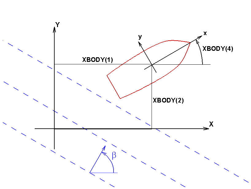
BETA is the array of wave heading angles in degrees. The wave heading is defined as the angle between the positive x-axis of the global coordinate system and the direction in which the waves propagate, as shown in Figure 4.1. The sign of the wave heading is defined by applying the right-hand rule to the body-fixed system. In POTEN the wave headings specified in the Potential Control File pertain to the solution of the diffraction problem only. If IDIFF= -1 NBETA should be set equal to 0 and no data BETA should be included in the POT file.
If NBETA< 0 a special convention is followed to assign a total of |NBETA| wave angles, with uniform increments, starting with the value equal to BETA(1) and using the increment equal to the value shown for BETA(2). In this case only two values BETA(1),BETA(2) should be included in the POT file. This option is convenient when a large number of uniformly spaced inputs are required. The two following examples show equivalent sets of input data in lines 7 and 8 of the POT file:
8 (NBETA)
0.0 45.0 90.0 135.0 180.0 225.0 270.0 315.0 (BETA array)
and
-8 (NBETA)
0.0 45.0 (BETA(1), increment)
NBODY is the number of bodies. Except for the analysis of multiple bodies (Chapter 8), NBODY=1.
GDF(K) is the name of the Geometric Data File of the Kth body.
XBODY(1,K), XBODY(2,K), XBODY(3,K) are the dimensional (X,Y,Z) coordinates of the origin of the body-fixed coordinate system of the kth body relative to the global coordinate system, as shown in Figure 4.1, in the same units of length as ULEN. The global coordinate system is required when walls are present (Section 12.4) and when multiple bodies are analyzed (Chapter 8). The global coordinate system is also used in place of the body coordinate system to define field-point data (fluid pressures, velocities, and free-surface elevation). Normally, in the absence of walls or multiple bodies, the coordinates XBODY(1) and YBODY(1) should be set equal to zero unless it is desired to refer the field-point data to a different coordinate system from that of the body. The incident-wave velocity potential is defined relative to the global coordinate system. Consequently, the phases of the exciting forces, motions, hydrodynamic pressure and field velocity induced by the incident wave are defined relative to the incident-wave elevation at X = Y = 0.
XBODY(4,K) is the angle in degrees of the x-axis of the body coordinate system of the Kth body relative to the X-axis of the global system, defined as positive in the counterclockwise sense about the vertical axis, as shown in Figure 4.1.
MODE is a six-element array of indices, assigned for each body, where I=1,2,3 correspond to the surge, sway and heave translational modes along the body-fixed (x,y,z) axes, and I=4,5,6 to the roll, pitch and yaw rotational modes around the same axes, respectively. Each of these six elements should be set equal to 0 or 1, depending on whether the corresponding radiation mode(s) and diffraction component(s) are required. (See the options IRAD=0 and IDIFF=0 above.)
The MODE array in the radiation solution specifies which modes of the radiation problem will be solved. To understand the significance of the MODE array in the diffraction solution, when symmetry planes are defined the complete diffraction problem is decomposed into symmetric/antisymmetric components in a manner which permits the most efficient solution, and when IDIFF=0, only those components of the diffraction potential required to evaluate the exciting force for the specified modes are evaluated. For example, if ISX=1, IDIFF=0, MODE(1)=1, and the remaining elements of MODE are set equal to zero, then the only component of the diffraction potential which is solved is that part which is antisymmetric in x. If the complete diffraction potential is required, for example to evaluate the drift forces or field data, IDIFF should be set equal to one.
4.3 THE FORCE CONTROL FILE (Alternative form 1)
The FRC file is used to input various parameters to the FORCE subprogram. The name of the FRC file can be any legal filename accepted by the operating system, with a maximum length of 16 ASCII characters, followed by the extension .frc.
In this Section the first form of the FRC file is described, in which the input of the body inertia matrix is simplified, and it is assumed that the body is freely floating.
Translation of the manual to HTML format can cause errors in file formating. Please see the PDF version of the manual for correct formmating.
The data in the Alternative 1 FRC file is listed below:
IOPTN(1) IOPTN(2) IOPTN(3) IOPTN(4) IOPTN(5) IOPTN(6) IOPTN(7) IOPTN(8) IOPTN(9)
VCG
XPRDCT(1,1) XPRDCT(1,2) XPRDCT(1,3)
XPRDCT(2,1) XPRDCT(2,2) XPRDCT(2,3)
XPRDCT(3,1) XPRDCT(3,2) XPRDCT(3,3)
NBETAH
BETAH(1) BETAH(2) ... BETAH(NBETAH)
NFIELD
XFIELD(1,1) XFIELD(2,1) XFIELD(3,1)
XFIELD(1,2) XFIELD(2,2) XFIELD(3,2)
XFIELD(1,3) XFIELD(2,3) XFIELD(3,3)
.
.
XFIELD(1,NFIELD) XFIELD(2,NFIELD) XFIELD(3,NFIELD)
The definition of each variable in the Force Control File is as follows:
‘header’ denotes a one-line ASCII header dimensioned CHARACTER*72. This line is available for the user to insert a brief description of the file, with a maximum length of 72 characters (including leading blanks).
IOPTN is an array of Option Indices. These indicate which hydrodynamic parameters are to be evaluated and output from the program. The available options, descriptions and filenames of the numeric output files are as follows:
| Option | Description | Filename |
| 1 | Added-mass and damping coefficients | frc.1 |
| 2 | Exciting forces from Haskind relations | frc.2 |
| 3 | Exciting forces from diffraction potential | frc.3 |
| 4 | Motions of body (response amplitude operator) | frc.4 |
| 5p | Hydrodynamic pressure on body surface | frc.5p |
| 5v | Fluid velocity vector on body surface | frc.(5vx,5vy,5vz) |
| 6p | Pressure/ free-surface elevation at field points | frc.6p |
| 6v | Fluid velocity vector at field points | frc .(6vx,6vy,6vz) |
| 7 | Mean drift force and moment from control surface | frc.7 |
| 8 | Mean drift force and moment from momentum | frc.8 |
| 9 | Mean drift force and moment from pressure | frc.9 |
The evaluation and output of the above parameters is in accordance with the following choice of the corresponding index:
IOPTN(I) = 0: do not output parameters associated with Option I.
IOPTN(I) = 1: do output parameters associated with Option I.
Options 2-9 may have additional values as listed below:
IOPTN(2) and IOPTN(3)
IOPTN(I) = 0: do not output the exciting forces
IOPTN(I) = 1: output the exciting forces
IOPTN(I) = 2: output the exciting forces and also the separate Froude-Krylov and scattering components of these forces (see Sections 3.3 and 5.3)
IOPTN(4)
IOPTN(4) = 0: do not output the response amplitude operator, RAO
IOPTN(4) = 1: output the RAO using the Haskind exciting force
IOPTN(4) = 2: output the RAO using the diffraction exciting force
IOPTN(4) = -3: output field data only for specified radiation modes
The use of IOPTN(4)=-1, -2, or -3 is explained in Section 4.5.
IOPTN(5)
IOPTN(5) = 0: do not output pressure and fluid velocity on the body
IOPTN(5) = 1: output pressure on the body
IOPTN(5) = 2: output fluid velocity on the body
IOPTN(5) = 3: output both pressure and fluid velocity on the body
IOPTN(6)
IOPTN(6) = 0: do not output pressure or velocity in the fluid and/or free-surface elevation
IOPTN(6) = 1: output pressure in the fluid and/or free-surface elevation by the potential formulation
IOPTN(6) = -1: output pressure in the fluid and/or free-surface elevation by the source formulation
IOPTN(6) = 2: output velocity in the fluid by the potential formulation
IOPTN(6) = -2: output velocity in the fluid by the source formulation
IOPTN(6) = 3: output both pressure and velocity in the fluid and/or free-surface elevation by the potential formulation
IOPTN(6) = -3: output both pressure and velocity in the fluid and/or free-surface elevation by the source formulation
IOPTN(7)
IOPTN(7) = 0: do not output the mean force and moment from control-surface integration
IOPTN(7) = 1: output the mean force and moment from control-surface integration only for unidirectional waves, using the potential formulation
IOPTN(7) = 2: output the mean force and moment from control-surface integration for all combinations of wave headings, using the potential formulation
IOPTN(7) = -1: output the mean force and moment from control-surface integration only for unidirectional waves, using the source formulation
IOPTN(7) = -2: output the mean force and moment from control-surface integration for all combinations of wave headings, using the source formulation
IOPTN(8)
IOPTN(8) = 0: do not output the mean force and moment from momentum integration
IOPTN(8) = 1: output the mean force and moment from momentum integration only for unidirectional waves
IOPTN(8) = 2: output the mean force and moment from momentum integration for all combinations of wave headings
IOPTN(9)
IOPTN(9) = 0: do not output the mean force and moment from pressure integration
IOPTN(9) = 1: output the mean force and moment from pressure integration only for unidirectional waves
IOPTN(9) = 2: output the mean force and moment from pressure integration for all combinations of wave headings
The options IOPTN(6)< 0 and IOPTN(7)< 0 apply only for the low-order method (ILOWHI=0), and require the source formulation (ISOR=1). If the low-order method is used the options IOPTN(5)>1 and IOPTN(9)>0 require the source formulation (ISOR=1).
The settings of the indices IOPTN(I) must be consistent with themselves and with the indices IRAD, IDIFF, and NBETA set in the Potential Control File. Error messages are generated if inconsistent indices are input. Otherwise, the indices IRAD, IDIFF and IOPTN(I), I=1,...,9 can be selected in any way the particular application may suggest. Three principal applications are as follows:
Forced motions in calm water (the radiation problem). In this case the modes of motion are specified by the MODE indices in the POT file. The diffraction index IDIFF should be set equal to -1. In the FRC file the indices IOTPTN(2:4) should be set equal to zero. The corresponding linear force coefficients are obtained with Option 1. Field pressures, velocities, free-surface elevations and drift forces follow from the corresponding Options 5-9.
Note that in the default case the pressures, velocities, and drift forces are not separated according to each mode, and the consequence of setting more than one mode to be nonzero is to superpose all such modes with unit amplitude. For example if IRAD=1 and IDIFF=-1, the default outputs from options 5-9 correspond to unit amplitudes of motion in all six degrees of freedom, with the same phase. Generally this is a nonphysical problem and care should be taken to avoid it. The simplest procedure to evaluate these outputs for each mode is to set MODE(I)=1 for only one mode. However this requires a separate run of WAMIT for each mode. It is possible to output separate results for options 5,6 for each mode of forced motion in a single run, using the configuration parameters INUMOPT5, INUMOPT6, as explained in Section 4.7.)
Diffraction of incident waves by a stationary structure (the diffraction problem). In this case the radiation index IRAD should be set equal to -1. To solve the complete diffraction problem set IDIFF=1, with corresponding outputs from the Options 3,5,6,7,8,9 in FORCE. (If IOPTN(4)=0 and IDIFF=1 it is assumed that the body is stationary, irrespective of IRAD. Thus, after a complete WAMIT run where the P2F file is output from POTEN and saved, it is possible to execute another run using only FORCE with the body motions both free and fixed, without re-running POTEN.)
Body motions in incident waves. In this case IRAD and IDIFF are set equal to 0 (body free only in specified modes) or 1 (body free in all modes). Body motions are obtained from the solution of the equations of motion using Option 4. The resulting field data and drift forces are evaluated for this particular combination of the radiation and diffraction solutions.
For bodies with one or two planes of symmetry (ISX=1 and/or ISY=1), the solution of the diffraction problem is decomposed into symmetric and antisymmetric components. If IDIFF=1 all of these components are computed, but if IDIFF=0 only the modes needed to evaluate the exciting forces corresponding to nonzero elements of the index IMODE in the POT file are computed. Special attention is necessary when computing the pressure, fluid velocity, and drift forces (Options 5-9), since these generally require all components of the diffraction solution. To ensure a complete solution, IDIFF=1 should be used in the POT file whenever Options 5-9 are computed. As explained in Section 5.8, a warning message is issued if IDIFF=0 and IOPTN(I)>0 for I=5-9, stating that the solution is non-physical. In special cases, where the heading angle coincides with a plane of symmetry, the complete diffraction solution is symmetric and it is not necessary to compute the antisymmetric component. In such cases the warning message can be ignored. This ‘shortcut’ is illustrated in Tests 06 and 14, where a TLP with two planes of symmetry is analyzed only in head seas (BETA=0), with IDIFF=0 and IMODE=0 for sway, roll and yaw; in this case the complete diffraction solution is symmetric about the plane Y=0, and the above inputs give correct results for Options 5-9.
VCG Dimensional z-coordinate of the center of gravity of the body relative to the origin of the body-system, input in the same units as the length ULEN.
XPRDCT is the 3 × 3 matrix of the body radii of gyration about the body-fixed axes, where I,J=1,2,3 correspond to (x,y,z) respectively, input in the same units as the length ULEN. More precisely, the elements of the body inertia matrix mij are evaluated for i,j = 4, 5, 6 according to the algorithm mij = m × XPRDCT(i - 3,j - 3) ×|XPRDCT(i - 3,j - 3)|. Here the body mass m is evaluated from the displaced mass of fluid, and the absolute value is used in the last factor so that negative products of inertia can be specified. The remaining elements of mij are evaluated assuming the body is freely floating in equilibrium, based on the calculated values of the displaced volume and center of buoyancy and on the specified value of VCG. In practical cases the matrix XPRDCT is symmetric. Zeroes may be specified if the body motions are not evaluated.
NBETAH is the number of Haskind wave headings, defined below. NBETAH must be an integer, greater than or equal to zero.
BETAH is an array of length NBETAH defined as the Haskind wave headings in degrees. The Haskind wave headings may be introduced in the Force Control File as an option, to enable evaluations to be made of the Haskind exciting forces (Option 2) and body motions in waves (Option 4) at heading angles not included in the Potential Control File. This option is feasible since the evaluation of Haskind exciting forces requires only the radiation potentials already determined by POTEN. This is a useful feature when the computational time is significant, since the time required to solve many diffraction problems in POTEN greatly exceeds the time required to evaluate the Haskind exciting forces in FORCE. Since the number of Haskind wave headings will affect the subsequent READ statements for data in the Force Control File, it is important to ensure that this number corresponds with the prescribed integer NBETAH. In particular, if NBETAH= 0 no values of BETAH should be included and NFIELD should appear on the next line of the Force Control File. If NBETAH> 0 is specified, the settings of the IOPTN switches are automatically set equal to 0 for options 3,5,6,7,8.
NFIELD is the number of points in the fluid domain (free surface) where the hydrodynamic pressure (wave elevation) and/or velocity are to be evaluated. NFIELD must be an integer, greater than or equal to zero.
XFIELD is a three-dimensional array with dimensions 3 ×NFIELD, defining the dimensional global coordinates of field points where the pressure/wave elevation and/or fluid velocity vector will be evaluated. Here I=1,2,3 correspond to the (X,Y,Z) coordinates. If Z = 0 the resulting output should be interpreted as the nondimensional wave elevation, otherwise as the nondimensional pressure. If NFIELD= 0 no input should be made for the array XFIELD.
Additional data is required to specify the field point array XFIELD when field points are placed inside internal tanks, as explained in Sections 4.7 and 12.1. When a large number of uniformly-spaced field points are required it is convenient to use the alternative inputs described in Section 4.11.
Starting in Version 7.1, the parameter TOLFPTWL is used to control the identification of field points on the free surface which are close to, or inside, body waterlines. If one or more field points on the free surface are inside a closed waterline, or within a nondimensional distance of the waterline which is less than TOLFPTWL, these points are identified as interior field points and the outputs for the hydrodynamic pressure and velocity are set equal to zero. In the supplementary output file frc.fpt the output 0 is appended on the line after the field point coordinates (see Section 5.2). An example of this output is included in Test05a. If TOLFPTWL≤ 0.0 is input in the cfg files the test of free surface field points is skipped.
When TOLFPTWL is used to test the locations of interior field points only closed waterlines with nonzero thickness are considered. Dipole panels/patches, wavemakers, and the waterlines of interior tanks are not included. Field points on the free surface of interior tanks are not included in this test. Users should verify the identification of interior field points, especially in cases where the shape of the waterline is unusual or irregular.
4.4 THE FORCE CONTROL FILE (Alternative form 2)
In this Section the second alternative form of the FRC file is described, where it is possible to specify separately three independent external force matrices including the mass matrix of the body, an external damping matrix, and an external stiffness matrix. This permits the analysis of bodies which are not freely floating in waves, with arbitrary linear external forces and moments, and also permits the specification of the complete body mass matrix instead of the simpler radii of gyration (cf. Section 4.3).
Translation of the manual to HTML format can cause errors in file formating. Please see the PDF version of the manual for correct formmating.
The format of the Alternative 2 FRC file is shown below:
IOPTN(1) IOPTN(2) IOPTN(3) IOPTN(4) IOPTN(5) IOPTN(6) IOPTN(7) IOPTN(8) IOPTN(9)
RHO
XCG YCG ZCG
IMASS
EXMASS(1,1) EXMASS(1,2) ... EXMASS(1,6+NEWMDS)
EXMASS(2,1) EXMASS(2,2) ... EXMASS(2,6+NEWMDS)
.
.
EXMASS(6+NEWMDS,1) EXMASS(6+NEWMDS,2) ... EXMASS(6,6+NEWMDS)
IDAMP
EXDAMP(1,1) EXDAMP(1,2) ... EXDAMP(1,6+NEWMDS)
EXDAMP(2,1) EXDAMP(2,2) ... EXDAMP(2,6+NEWMDS)
.
.
EXDAMP(6+NEWMDS,1) EXDAMP(6+NEWMDS,2) ... EXDAMP(6,6+NEWMDS)
ISTIF
EXSTIF(1,1) EXSTIF(1,2) ... EXSTIF(1,6+NEWMDS)
EXSTIF(2,1) EXSTIF(2,2) ... EXSTIF(2,6+NEWMDS)
.
.
EXSTIF(6+NEWMDS,1) EXSTIF(6+NEWMDS,2) ... EXSTIF(6+NEWMDS,6+NEWMDS)
NBETAH
BETAH(1) BETAH(2) ... BETAH(NBETAH)
NFIELD
XFIELD(1,1) XFIELD(2,1) XFIELD(3,1)
XFIELD(1,2) XFIELD(2,2) XFIELD(3,2)
XFIELD(1,3) XFIELD(2,3) XFIELD(3,3)
.
.
XFIELD(1,NFIELD) XFIELD(2,NFIELD) XFIELD(3,NFIELD)
The header, IOPTN array, and all lines beginning with the variable NBETAH, are identical to the data in the Alternative form 1 FRC file. The data which differ in Form 2 are described below.
RHO Dimensional density of the fluid, in the same units as used for the external force matrices and for GRAV.
XCG YCG ZCG Dimensional coordinates of the body center of gravity in terms of the body coordinate system and in the same units as ULEN.
IMASS This index is either 0 or 1, to signify if the external mass matrix EXMASS is read. If the value of the index is zero, the matrix EXMASS is not included in the FRC file and the program assumes that all values in this matrix are zero. If the value of the index is one, the matrix EXMASS is included in the FRC file.
EXMASS is the (6+NEWMDS) × (6+NEWMDS) dimensional inertia matrix of the body about the body-fixed axes. (For a conventional rigid body this is a 6 × 6 dimensional matrix as defined in Reference [3], page 149, equation 141.) Each element in this matrix is added to the corresponding added mass of the body, in setting up the equations of body motions.
IDAMP This index is either 0 or 1, to signify if the external damping matrix EXDAMP is read. If the value of the index is zero, the matrix EXDAMP is not included in the FRC file and the program assumes that all values in this matrix are zero. If the value of the index is one, the matrix EXDAMP is included in the FRC file.
EXDAMP is the (6+NEWMDS) × (6+NEWMDS) dimensional damping matrix of an arbitrary external force or moment acting on the body, e.g. from a mooring cable subject to viscous damping. The value of each element in this matrix is added to the corresponding linear wave damping coefficient of the body, in setting up the equations of body motions.
ISTIF This index is either 0 or 1, to signify if the external mass matrix EXSTIF is read. If the value of the index is zero, the matrix EXSTIF is not included in the FRC file and the program assumes that all values in this matrix are zero. If the value of the index is one, the matrix EXSTIF is included in the FRC file.
EXSTIF is the (6+NEWMDS) × (6+NEWMDS) dimensional stiffness matrix of an arbitrary external force or moment acting on the body, e.g. from an elastic mooring cable. In setting up the equations of body motions, the value of each element in this matrix is added to the corresponding restoring coefficient of the body, including both hydrostatic pressure and the gravitational moment due to the body’s mass, as defined in Section 3.1. (The vertical inertia force due to heave, EXMASS(3,3), is assumed equal to the body mass and is used to derive the gravitational restoring moment of the body. In any situation where this assumption is not satisfied, due to the presence of an external vertical inertia force, the gravitational restoring moment should be corrected for this difference via the stiffness matrix EXSTIF.)
The units of EXMASS, EXDAMP, EXSTIF must correspond to those used to specify the fluid density RHO and the length ULEN, with time measured in seconds. These matrices must be defined with respect to the body-fixed coordinate system.
It is also possible to use Alternative Form 2 with the external force matrices in separate files. In this case the index IMASS, IDAMP, and/or ISTIF is set equal to 2, and followed by the corresponding file name:
IOPTN(1) IOPTN(2) IOPTN(3) IOPTN(4) IOPTN(5) IOPTN(6) IOPTN(7) IOPTN(8) IOPTN(9)
RHO
XCG YCG ZCG
2
MASS (file name containing inertia matrix)
2
DAMP (file name containing damping matrix)
2
STIF (file name containing stiffness matrix)
NBETAH
BETAH(1) BETAH(2) ... BETAH(NBETAH)
NFIELD
XFIELD(1,1) XFIELD(2,1) XFIELD(3,1)
XFIELD(1,2) XFIELD(2,2) XFIELD(3,2)
XFIELD(1,3) XFIELD(2,3) XFIELD(3,3)
.
.
XFIELD(1,NFIELD) XFIELD(2,NFIELD) XFIELD(3,NFIELD)
MASS is a file name which contains external inertial forces to the bodies and interactive inertial forces between bodies. For example, the data in MASS for a body are listed below:
EXMASS(1,1) EXMASS(1,2) ... EXMASS(1,6+NEWMDS)
EXMASS(2,1) EXMASS(2,2) ... EXMASS(2,6+NEWMDS)
.
.
EXMASS(6+NEWMDS,1) EXMASS(6+NEWMDS,2) ... EXMASS(6+NEWMDS,6+NEWMDS)
For N interacting bodies, the number of data in MASS are NDFR × NDFR, where NDFR=∑ n=1N(6 + NEWMDS(n)) is the total number of rigid body modes and generalized modes. Similarly the external damping and stiffness can be specified to the files DAMP and STIF. In summary, there are three legal values for IMASS, IDAMP, ISTIFF:
I=0: no matrix or file name is input, matrix is assumed equal to zero
I=1: matrix follows on subsequent lines
I=2: file name follows on next line
The procedure to designate Alternative Form 2 is to assign the parameter IALTFRC=2 in the configuration file, as described in Section 4.7, and use the formats above. In early versions of WAMIT the parameter IALTFRC was assigned differently, by inserting the integer 2 on a separate line after the header line of the FRC file. This variant of the FRC file format was supported in Version 6. Version 7 issues an error message if this variant is input.
4.5 DEFINITION OF FIXED OR FREE MODES
Translation of the manual to HTML format can cause errors in file formating. Please see the PDF version of the manual for correct formmating.
It is possible to specify that a sub-set of the modes of body motion analyzed in POTEN can be fixed in FORCE. As a simple example, consider a single body with six degrees of rigid-body motions, all of which have been analyzed in POTEN (either by setting IRAD=1 or by setting IRAD=0 and setting all six elements of MODE=1). Normally, in the FORCE analysis, if (IOPTN(4)>0, the body motions are computed for all degrees of freedom. Now suppose that the body is restrained in the vertical modes (heave, roll, pitch) as would be the case for the first-order motions of a tension-leg platform. This condition can be analyzed in FORCE by modifying the Force Control File in the following manner:
(1) assign a negative value to IOPTN(4) (-1 to use the Haskind exciting force or -2 to use the diffraction exciting force).
(2) insert two new lines of data after IOPTN (before VCG or RHO):
MODE(1),MODE(2),MODE(3), ... MODE(NDFR)
Here NDFR is the total number of possible radiation modes and MODE is an array with the value of each element 0 if the mode is fixed or 1 if the mode is free. For the example described above, NDFR=6 and MODE = (1,1,0,0,0,1). Thus surge, sway, and yaw are free while heave, roll, and pitch are fixed.
When this option is employed the RAO’s output for the free modes are defined in the conventional manner, as the amplitudes of body motions in the corresponding degrees of freedom. For the fixed modes the RAO’s are replaced by the loads acting on the body in the corresponding directions. In this case the corresponding modal index in the output file is shown with a negative value, to signify the change. For the example described above, the output RAO for heave is equal to the vertical load acting on the body (equal and opposite to the load on the restraining structure), and preceded by the index -3. The TLP Test Runs (06 and 14) described in the Appendix illustrate this application.
For a single body with no generalized modes NDFR=6 in all cases. For the analysis of multiple bodies (cf. Chapter 8), with no generalized modes, NDFR=6*NBODY. If generalized modes are analyzed (cf. Chapter 9) NDFR is the total number of modes for all bodies, including both rigid-body modes and generalized modes. Thus, in the most general case, NDFR=6*NBODY+∑ n=1NBODY NEWMDS(n).
If fixed/free modes are specified for multiple bodies, using IALTFRC=3 as described in Section 8.3, the modifications (1) and (2) described above must be included only in the Global Force Control File (GFRC) and not in the separate Force Control Files for each body.
It is also possible to perform the analysis in FORCE for a problem where no incident waves exist, after running POTEN with incident waves present and with the diffraction solution obtained. To suppress the incident waves in FORCE, IOPTN(4)=-3 is assigned in the FRC file. In that case the body pressure/velocity, field point pressure/velocity, and mean drift forces are evaluated assuming that the body is oscillating in the specified free mode(s), without incident waves.
4.6 BODY PRESSURE AND FLUID VELOCITY AT SPECIFIED POINTS
Translation of the manual to HTML format can cause errors in file formating. Please see the PDF version of the manual for correct formmating.
If IOPTN(5)> 0 the points on the body surface where the pressure and fluid velocity are evaluated depend on the parameter IPNLBPT in the configuration file. In the default case IPNLBPT=0, these points are at the panel centroids in the low-order method (ILOWHI=0) or at a set of uniformly-spaced parametric points on each patch in the higher-order method (ILOWHI=1).
If IPNLBPT≠0 the body pressure is evaluated at points on the body which are specified by the user in a special input file gdf.bpi (Body Point Input). The format of this file is as follows:
NBPT
X(1) Y(1) Z(1)
X(2) Y(2) Z(2)
.
.
X(NBPT) Y(NBPT) Z(NBPT)
The filename of this file must be the same as the filename of the GDF file.
If IPNLBPT> 0, the data in the .bpi file is read and interpreted to be in dimensional body-fixed coordinates. If IPNLBPT< 0, the data in the .bpi file is read and interpreted to be in dimensional global coordinates.
The procedure used to evaluate the body pressure at these specified points is different in the low-order (ILOWHI=0) and higher-order (ILOWHI=1) solutions. These are described separately below.
If ILOWHI=0, the solution is based on piecewise constant values of the potential on each panel based on colocation at the panel centroids. In order to evaluate the pressure at other points an interpolation procedure is adopted. This interpolation is based on the absolute value of the input parameter IPNLBPT. IPNLBPT=4 is recommended, when the input points are in body-fixed coordinates. In this case the program searches and identifies the four nearest panel centroids to each specified input point, and assigns weights to each of these panels based on the (inverse) distance to each centroid.
In the higher-order method (ILOWHI=1) the solution for the velocity potential and pressure is represented by continuous B-splines on each patch. For each specified input point (x,y,z) the program searches for the patch index and parametric coordinates (U,V ) of the point on this patch which is closest to the input point. The pressure and velocity are evaluated at the corresponding point (U,V ). An iterative procedure is used to find (U,V ), with a specified convergence tolerance of 1.0E-4 for the radial distance in nondimensional Cartesian coordinates. (When the length scale of the patch is larger than 1.0 the tolerance is increased by a factor equal to this length scale, estimated from the Jacobian of the parametric transformation at the center of the patch.) A warning message is generated if nonconvergence occurs for one or more input points, showing the total number of unconverged points. (See also Section 5.5.)
The pressure and velocity are output in the .5p and .5v* files as explained in Section 5.5. Data related to the coordinates of the evaluation points are tabulated in the supplementary output file gdf.bpo which is explained in the same Section.
In both the low-order and higher-order implementations, the input data in the .bpi file should correspond to points which lie as close as possible to the body surface. If points in the BPI files are very close to intersections of adjacent patches in the higher-order method, the index NP in the BPO file should be checked to verify that the correct patch is used, especially in cases where there is ambiguity between the pressure on a conventional patch and the pressure jump on a dipole patch. Similarly, in the low-order method, the panel indices, N1, N2, ... in the BPO file can be checked to verify the corresponding output at the points in BPI files is the pressure obtained from those on the conventional body panels or the pressure jump on the dipole panels.
4.7 CONFIGURATION FILES ‘CONFIG.WAM’ AND ‘*.CFG’
Two optional configuration files may be used to specify various parameters and options in WAMIT. The first configuration file is assigned the reserved name config.wam. The second filename is specified by the user, with the extension ‘.cfg’. Both files are opened and read, if they exist, and the configuration parameters defined below can be included in either the first or second file. It is recommended to use the first file for parameters which are the same for most or all applications, and to use the second file for parameters which depend on the specific run. If the same parameter is defined in both files, the input from the second is used for the run. If the second configuration file is used its complete filename including the extension ‘.cfg’ must be included in the input file fnames.wam. The test runs listed in Appendix A show examples of these conventions.
The inputs which may be specified in the configuration files are as follows:
| Parameter | Default value | |
| CHANNEL_WIDTH | -1.0 | |
| CHANNEL_REFLECT | 1.0 | |
| IALTCSF | 1 | |
| IALTFRC | 1 | |
| IBODYW | 0 | |
| ICCFSP | 0 | |
| IDAMPER | 0 | |
| IDELFILES | 0 | |
| IFIELD_ARRAYS | 0 | |
| IFORCE | 1 | |
| IGENMDS | 0 | |
| ILOG | 0 | |
| ILOWGDF | 0 | |
| ILOWHI | 0 | |
| IMODESFSP | ||
| INUMOPT5 | 0 | |
| INUMOPT6 | 0 | |
| IOUTFNAME | 0 | |
| IOUTLOG | 0 | |
| IPERIN | 1 | |
| IPEROUT | 1 | |
| IPLTDAT | 0 | |
| IPLTFEPOINT | 0 | |
| IPLTNORMAL | 0 | |
| IPNLBPT | 0 | |
| IPOTEN | 1 | |
| IQUADI† | 4 | |
| IQUADO† | 3 | |
| IREADRAO | 0 | |
| IRR | 0 | |
| ISCATT | 0 | |
| ISOLVE | 0 | |
| ISOR | 0 | |
| ITANKFPT | 0 | |
| ITRIMWL | 0 | |
| IWALLX0 | 0 | |
| IWALLY0 | 0 | |
| KSPLIN† | 3 | |
| MAXITT | 35 | |
| MAXMIT | 8 | |
| MODLST | 0 | |
| MONITR | 0 | |
| NCPU | 1 | |
| NEWMDS | 0 | |
| NFIELD_LARGE | 0 | |
| NMODESFSP | 0 | |
| NOOUT | 1 | |
| NPDIPOLE | ||
| NPFORCE | ||
| NPFSP | ||
| NPNOFORCE | ||
| NPTANK | ||
| NUMHDR | 0 | |
| NUMNAM | 0 | |
| PANEL_SIZE | -1.0 | |
| PLTDELTA | 0.05 | |
| RAMGBMAX | 0.5 | |
| RHOTANK | ||
| SCRATCH_PATH | current directory | |
| TOLFPTWL | 1.E-3 | |
| TOLGAPWL | 1.E-3 | |
| USERID_PATH | current directory | |
| VMAXOPT9 | -1.0 | |
| XTRIM | ||
| ZTANKFS | ||
These parameters only need to be included when they are required. Parameters where a specified default value is shown are assigned this value when the parameter is not included explicitly. The parameters marked † are spline control parameters defined in Sections 7.11-12. These can be input either in the .cfg or .spl file.
When multiple bodies are analyzed (NBODY>1) there are additional parameters, and some of the parameters in the list above must be assigned with separate values for each body (See Section 8.4).
Explanations of the parameters which may be specified in the configuration file are as follows:
CHANNEL_WIDTH is a parameter which can be used to define the width of a channel with parallel walls, as explained in Section 12.7. If this parameter is used it should have a positive real value. Zero or a negative value is interpreted to mean that the width of the fluid domain is infinite. The default value is CHANNEL_WIDTH = -1.0
CHANNEL_REFLECT is a parameter which can be used to reduce the effect of wave reflection from parallel walls, as explained in Section 12.7. If this parameter is used it must be in the range between zero and one. The default value is CHANNEL_REFLECT = 1.0.
IALTCSF is an integer specifying the alternative methods of evaluating the mean drift force and moment using a control surface, as explained in Chapter 11 and Section 15.9.
IALTCSF= 1: use Alternative 1
IALTCSF= 2: use Alternative 2
The default value is IALTCSF=1.
IALTFRC is an integer specifying the alternative forms of the FRC file as explained in Sections 4.3, 4.4, and 8.3-5.
IALTFRC= 1: use the Alternative Form 1 FRC format shown in Section 4.3,
IALTFRC= 2: use the Alternative Form 2 FRC format shown in Section 4.4,
IALTFRC= 3: use the Alternative Form 3 FRC format shown in Section 8.5.
The default value is IALTFRC=1.
IBODYW is an integer specifying the body number of the first body which represents a wavemaker in a wall (see Section 12.3).
The default value is IBODYW= 0: No wavemakers are present in walls.
ICCFSP is an integer specifying the option to exclude or include the external restoring coefficients due to the pressure acting on closed chambers above free-surface pressure surfaces (see Section 12.5).
The default value is ICCFSP= 0: Do not include the external restoring coefficients.
IDAMPER is an integer specifying the option to use fluid damping surfaces as explained in Section 12.8.
IDAMPER= 1: free damper, impervious
IDAMPER= 2: fixed damper, porous
IDAMPER= 3: free damper, porous
IDAMPER= -1: free damper, impervious, generalized-mode method
The default value is IDAMPER=0.
IDELFILES is an integer specifying the option to delete and overwrite old output files with the same filenames, as explained in Section 5.1 and Section 5.10.
IDELFILES= 1: overwrite old P2F file without interactive prompt,
IDELFILES= 2: overwrite old P2F and OUT files without interactive prompts,
IDELFILES= 3: overwrite old P2F file and delete new P2F file,
IDELFILES= 4: overwrite old P2F and OUT files and delete new P2F file.
The default value is IDELFILES=0.
IFIELD_ARRAYS is an integer parameter specifying if uniform arrays of field points are assigned in the FRC control file, using a compressed format as explained in Section 4.11.
IFIELD_ARRAYS= 0: Field point data is assigned only as shown in the conventional FRC files, as explained in Sections 4.3 and 4.4.
IFIELD_ARRAYS= 1: Additional field point data is assigned in the conventional FRC files, as explained in Section 4.11.
The default value is IFIELD_ARRAYS= 0.
IFORCE is an integer parameter specifying if the FORCE subprogram is executed during the WAMIT run.
IFORCE= 0: Do not execute FORCE.
IFORCE= 1: Execute FORCE.
IFORCE= 2: Execute FORCE and POTEN simultaneously for each wave period (see Section 4.14).
The default value is IFORCE= 1.
IGENMDS is an integer parameter specifying the option to input the geomeric data associated with the mode shapes of generalized modes, when NEWMDS > 0. The details on the use of the generalized mode option are described in Chapter 9.
IGENMDS= 0: use a seperate program DEFMOD to input the geometric data for generalized modes. This option can be used only with the low order method (ILOWHI=0). In this case the user prepares a subroutine in DEFINE to describe the generalized mode shapes.
IGENMDS≠0: use a DLL file containing the subroutine NEWMODES. The user modifies NEWMODES to specify the mode shape. This option can be used with both the low- and higher-order options.
The default value is IGENMDS= 0.
ILOG is an integer parameter specifying the option to integrate the logarithmic singularity in the Green function separately, with a more accurate numerical integration scheme.
ILOG= 0: The logarithmic singularity is included with the wavelike component of the Green function and is integrated by quadrature over each panel or patch.
ILOG= 1: The logarithmic singularity in the Green function is subtracted and integrated in a similar manner as the Rankine image singularity 1∕r′. (This option produces more accurate results.)
The default value is ILOG= 0.
ILOG=1 is required when panels or patches are defined in the plane of the free surface, including the following two cases: (1) bodies with horizontal physical surfaces lying in the plane of the free surface, and (2) use of the irregular frequency option, where panels are located on the interior free surface inside the body waterline. In these two cases, execution of the program is interrupted with an error message if ILOG=0.
ILOWGDF is an integer parameter specifying the option to generate a low-order GDF output file based on the input geometry (see Section 5.7). If ILOWHI=0, the original input panels are used. If ILOWHI=1 the low-order output panels are generated from the panels of the higher-order geometry. If ILOWGDF> 1, the panels are subdivided into ILOWGDF×ILOWGDF sub-panels.
ILOWGDF= 0: Do not generate the output file gdf_LOW.GDF.
ILOWGDF≥ 1: Generate the output file gdf_LOW.GDF.
The default value is ILOWGDF= 0.
ILOWHI is an integer parameter specifying the use of the low-order or higher-order panel method.
ILOWHI= 0: Low-order panel method (Chapter 6)
ILOWHI= 1: Higher-order panel method (Chapter 7)
IMODESFSP is an integer parameter specifying the subroutine used to define pressure distributions on interior free surfaces of the body (see Section 12.5).
INUMOPT5 is an integer parameter specifying the option to evaluate the separate radiation and diffraction components of the body pressure and velocity (see Sections 3.5 and 3.7).
INUMOPT5= 0: output the total body pressure and velocity.
INUMOPT5= 1: output the total body pressure and velocity in the formatted output file (.out). Output the separate components in the numeric output files (.5p, .5vx, .5vy, .5vz).
INUMOPT6 is an integer parameter specifying the option to evaluate the separate radiation and diffraction components of the pressure and velocity at field points (see Sections 3.5 and 3.7).
INUMOPT6= 0: output the total field pressure and velocity.
INUMOPT6= 1: output the total field pressure and velocity in the formatted output file (.out). Output the separate components in the numeric output files (.6p, .6vx, .6vy, .6vz).
IOUTFNAME is an integer parameter specifying the filename of the output files (see Section 5.1).
IOUTFNAME= 1: Append _N to the filename (1 ≤ N ≤ 9)
IOUTFNAME= 2: Append _NN to the filename (1 ≤ NN ≤ 99)
IOUTFNAME= 3: Append _NNN to the filename (1 ≤ NNN ≤ 999)
IOUTFNAME= 4: Append _NNNN to the filename (1 ≤ NNNN ≤ 9999)
The default value is IOUTFNAME= 0.
IOUTLOG is an integer parameter specifying the option to save a copy of the log file wamitlog.txt with the filename of the output files (see Section 5.9).
IOUTLOG= 1: Save a copy of the log file with the filename of the output files
The default value is IOUTLOG= 0.
IPERIN is an integer parameter specifying the input data for PER in the POT file (see Section 4.2).
IPERIN= 1: Input periods in seconds
IPERIN= 2: Input radian frequencies
IPERIN= 3: Input infinite-depth wavenumbers
IPERIN= 4: Input finite-depth wavenumbers
The default value is IPERIN= 1.
(The use of IPERIN is identical to the parameter IPERIO in Version 6. The name of this parameter is changed in Version 7 to correspond with the parameter IPEROUT.)
IPEROUT is an integer parameter specifying the output data for PER. The same four optional values IPEROUT= 1, 2, 3, 4 are used as defined above for the corresponding input parameter IPERIN. The default value is IPEROUT= 1. IPEROUT controls the first column of data in the numeric output files, and also the first column of data in the header of the OUT file showing the runtimes and iterations for the POTEN run, as well as the same runtime outputs to the monitor during the POTEN run.
IPLTDAT is an integer parameter specifying the option to generate the output files gdf_PAN.DAT and gdf_PAT.DAT, used for plotting the panel and patch discretizations (see Section 5.7).
IPLTDAT= 0: Do not generate the output files gdf_PAT.DAT and gdf_PAN.DAT
IPLTDAT≥ 1: Generate the output files gdf_PAT.DAT and gdf_PAN.DAT for plotting the panel and patch discretizations with IPLTDAT×IPLTDAT subdivisions.
The default value is IPLTDAT= 0.
IPLTFEPOINT is an integer parameter specifying the option to generate the output file gdf_PAN.DAT in POINT or FEPOINT format (see Section 5.7). This option is only available when the higher-order method is used (ILOWHI=1).
IPLTFEPOINT= 0: Generate the output file gdf_PAN.DAT using POINT format
IPLTFEPOINT= 1: Generate the output file gdf_PAN.DAT using FEPOINT format
The default value is IPLTFEPOINT= 0.
IPLTNORMAL is an integer parameter specifying the option to show the interior normal vectors in the output files gdf_PAN.DAT and gdf_PAT.DAT
IPLTNORMAL= 0: Do not include data to show the normals
IPLTNORMAL= 1: Show projected panels/patches to indicate the direction of the normal vectors
IPLTNORMAL= 2: Show the normal vectors on each panel/patch
The default value is IPLTNORMAL= 0.
IPNLBPT is an integer parameter specifying the option to evaluate the body pressure at specified points (x,y,z) listed in the input file gdf.BPI.
IPNLBPT= 0: output the body pressure at the panel centroids, or on a uniform parametric mesh in the higher-order method.
IPNLBPT≥ 1: output the body pressure at the points listed in the input file gdf.BPI. These points are defined with reference to the body-fixed dimensional Cartesian coordinates for each body.
IPNLBPT≤-1: output the body pressure at the points listed in the input file gdf.BPI. These points are defined with reference to the global coordinate system.
The default value is IPNLBPT= 0. When IPNLBPT≠0 and ILOWHI=0, the absolute value of IPNLBPT specifies the number of panels nearest to each point specified in gdf.BPI. See Section 4.6 for further details.
IPOTEN is an integer parameter specifying if the POTEN subprogram is executed during the WAMIT run.
IPOTEN= 0: Do not execute POTEN.
IPOTEN= 1: Execute POTEN.
The default value is IPOTEN= 1.
IQUADI is an integer parameter specifying the order of the inner Gauss quadrature parameter IQUI for all patches when the higher-order method is used (ILOWHI=1). The default value is IQUADI=4. (See Sections 7.11-12.)
IQUADO is an integer parameter specifying the order of the outer Gauss quadrature parameter IQUO for all patches when the higher-order method is used (ILOWHI=1). The default value is IQUADO=3. (See Sections 7.11-12 for further information.)
IREADRAO is an integer parameter specifying if the RAO’s are to be input from an external file, as explained in Section 4.3.
IREADRAO= 0: Use RAO’s computed by WAMIT in Option 4 to evaluate Options 5-9
IREADRAO= 1: Evaluate only Options 1,2,3,4
IREADRAO= 2: Read RAO’s in complex format from an external file to evaluate Options 5-9
IREADRAO= 3: Read RAO’s from modulus and phase in an external file to evaluate Options 5-9
The default value is IREADRAO=0.
IRR is the integer used to specify whether the irregular frequencies are removed. The use of IRR is described in Chapter 10.
IRR= 0: Do not remove the effect of the irregular frequencies.
IRR= 1: Remove the effect of the irregular frequencies. (User needs to represent the interior free surface by panels or patches.)
IRR= 2: Remove the effect of the irregular frequencies. (Program projects the body panels on the interior free surface.) This option is restricted to the low-order method (ILOWHI=0).
IRR= 3: Remove the effect of the irregular frequencies. (Program automatically discretizes the interior free surface.)
The default value is IRR=0.
ISCATT is an integer parameter specifying whether the diffraction or the scattering problem is solved to obtain the diffraction potential. The diffraction potential may be solved by the equation (15.12) which we define as the diffraction problem. Alternatively in the scattering problem, the scattered potential is solved by (15.13) and the diffraction potential is obtained from equation (15.8): This option is only available in the low-order method (ILOWHI=0).
ISCATT= 0: Solve the diffraction problem
ISCATT= 1: Solve the scattering problem
The default value is ISCATT=0.
ISOLVE is an integer parameter specifying the method of solution for the linear systems in POTEN. These three alternative methods are described in Section 14.2.
ISOLVE=0: Use the iterative solver
ISOLVE= 1: Use the direct solver
ISOLVE= N (N ≥ 2) : Use the block iterative solver with N blocks
ISOLVE= -1 Special value used for wavemakers in planes of symmetry (See Section 12.3)
The default value is ISOLVE=0.
ISOR is the integer used to specify whether the source strength is evaluated:
ISOR=0: Do not evaluate the source strength.
ISOR= 1: Evaluate the source strength.
The default value is ISOR=0.
The source strength is required in the low-order method (ILOWHI=0) if FORCE evaluates the fluid velocity on the body (IOPTN(5)=2 or 3), the pressure/free-surface elevation or velocity in the fluid domain by the source formulation (IOPTN(6)<0) and the mean drift force and moment from pressure integration (IOPTN(9)=1 or 2). For the control-surface drift force and moment (IOPTN(7)=1 or 2), if ISOR=0, only the horizontal drift force and vertical moment can be evaluated using Alternative 1 (IALTCSF=1); ISOR=1 is required for the other components using Alternative 1, and for all components using Alternative 2. Running POTEN with ISOR=1 requires substantially longer run time and larger scratch storage. In the higher-order method (ILOWHI=1) all of the FORCE evaluations are made directly from the solution for the velocity potential, and ISOR=0 is required.
ITANKFPT is an integer parameter specifying the option to input field point (fpt) coordinates in the .frc control file, either in the conventional format (default) or in the format required when some or all of the field points are located within internal tanks. The default value ITANKFPT=0 should be used except in cases where tanks are included with field points inside the tanks.
ITANKFPT=0: All field points are in the exterior domain. Field points are input as specified in Sections 4.3 and 4.4, with the coordinates of each field point on one line, or using the array format described in Section 4.11.
ITANKFPT= 1: Field points are listed in the .frc control file with the tank number preceding the coordinates. Thus, in place of the XFIELD lines shown in Section 4.3, the correponding data are input as follows:
ITANK(n) XFIELD(1,n) XFIELD(2,n) XFIELD(3,n)
ITANK(n) is an integer which specifies the tank number containing the n’th field point. If ITANK(n)=0, the field point is in the exterior domain. The numbering of the tanks corresponds to the order of the NPTANK indices, as explained below.
The default value is ITANKFPT=0.
ITRIMWL is the integer parameter used to specify the trimmed-waterline option (See Section 12.2). When ITRIMWL>0 the array XTRIM must be included for each body.
The default value is ITRIMWL=0.
IWALLX0 is the integer parameter used to specify that the plane X=0 is a reflecting wall (See Section 12.4). When IWALLX0=1 the fluid is bounded by a reflecting wall at X=0.
The default value is IWALLX0=0.
IWALLY0 is the integer parameter used to specify that the plane Y=0 is a reflecting wall (See Section 12.4). When IWALLY0=1 the fluid is bounded by a reflecting wall at Y=0.
The default value is IWALLY0=0.
KSPLIN is an integer parameter specifying the value of the B-spline orders KU,KV for all patches when the higher-order method is used (ILOWHI=1). The default value is KSPLIN=3. (See Sections 7.11-12 for further information.)
MAXITT is an integer parameter used to specify the maximum number of iterations in the iterative solver (See Section 14.2).
The default value MAXITT=35 is recommended for general use.
MAXMIT is the maximum number of iterations in the adaptive integration used to evaluate the momentum integral for the drift force and moment (Option 8). (The maximum number of integration ordinates in the azimuthal direction is 2MAXMIT .) The default value MAXMIT=8 is assigned unless a different value is input in the CFG file; this value is recommended for general use.
MODLST is the integer parameter used to control the order in which the added-mass and damping coefficients, exciting forces, and RAO’s for different modes of motion are written to the output files. MODLST=0: Outputs are in ascending order of the modal indices.
MODLST= 1: Outputs are in the order evaluated for each of the corresponding left-hand-sides.
These two alternatives differ only if NLHS is greater than one. The default value is MODLST=0.
MONITR is the integer parameter used to control the display of output to the monitor during the execution of FORCE.
MONITR=0: Outputs to the monitor are abbreviated, consisting of the header text and displays of each wave period as it is executed. This option is convenient in long runs of FORCE with extensive lines of output, to permit monitoring the progress of the execution.
MONITR= 1: Outputs of all data evaluated by FORCE are displayed on the monitor during execution, in the same format as in the OUT file.
The default value is MONITR=0.
NCPU is an integer which specifies the number of parallel processors (CPU’s, also known as ‘cores’) which are available on the system. The default value NCPU=1 is applicable for most older PC’s. The use of NCPU>1, when this is available on the system, permits substantial reduction in run times (See Section 14.6).
NEWMDS is an integer parameter specifying the number of generalized modes for each body. The default value is NEWMDS=0. (See Chapter 9.)
NFIELD_LARGE is an integer parameter specifying the option to evaluate the hydrodynamic pressure and/or velocity at very large arrays of field points, separately from the other outputs, as explained in Section 14.9.
NFIELD_LARGE= 0: Field outputs are evaluated in the period loop with other FORCE outputs.
NFIELD_LARGE= 1: Field outputs are evaluated in a separate loop after the other FORCE outputs.
The default value is NFIELD_LARGE= 0.
NMODESFSP is an integer array used to specify the number of modes used to define the pressure distribution on free-surface pressure surfaces. Further details are given in Section 12.5.
NOOUT is an integer array with length 9, used to control the output to the OUT file. Each element of the array corresponds to one of the 9 options in FRC. If the element equals 0, the corresponding output is omitted from the OUT file.
NOOUT(I)=0 Omit the output corresponding to IOPTN(I) in the OUT file
NOOUT(I)= 1 Include the output corresponding to IOPTN(I) in the OUT file
If NOOUT is included in the configuration file all 9 integers must be specified. An example is shown on the next line, which specifies that all outputs are included in the OUT file except the pressures and/or fluid velocities on the body panels.
NOOUT= 1 1 1 1 0 1 1 1 1
This option can be useful to avoid very long OUT files, since the data for option 5 is generally much more extensive than for the other options. The default value NOOUT(I)= 1 for I = 1,..., 9 is assigned if NOOUT is not included in the configuration file. (The data for each specified option is always included in the corresponding numeric output file, regardless of the array NOOUT.)
NPDIPOLE is an integer array used to specify the panel or patch indices of zero-thickness elements represented by dipoles. Multiple lines of input can be used, but each line must begin with ‘NPDIPOLE =’. The data on these lines may specify either individual indices of each dipole panel/patch, or ranges of consecutive indices which are indicated by enclosing a pair of indices in parenthesis. The following three examples are equivalent ways of specifying that the indices 2, 4, 5, 6, 8 are dipole panels or patches:
NPDIPOLE= 2 4 5 6 8
NPDIPOLE= 2 (4 6) 8
NPDIPOLE= (2 2) (4 6) (8 8)
Note that parenthesis must be used to denote the lower and upper limits of a range of consecutive indices, and parentheses must not be used for any other purpose. Other ASCII characters may be included on these lines, and are ignored. It is not necessary for the individual indices or ranges to be in ascending order, except for the first and last indices of each range enclosed in parentheses.
The Version 6 option to define dipole panels or patches in the GDF file is not supported in Version 7.
NPFORCE is an integer array used to specify the panels or patches which are included in the integrations of the pressure force and moment. The data in this array are in pairs, with the same format rules as specified below for NPFSP. Further details are given in Section 12.6.
NPFSP is an integer array used to specify the panel or patch indices of free-surface pressure surfaces. The data in this array are in pairs, denoting the first and last index for each surface. An even number of indices must be included on each line. Each pair of indices must be enclosed in parentheses, as shown in the input file test25.cfg. More than one line can be used for multiple surfaces, and/or multiple surfaces can be defined on the same line. Only integer data and parentheses are read for the array NPFSP, with spaces or other characters separating each index. Other ASCII characters may be used in addition to the integers and parenthesis, but integers and parenthesis must be used only for the inputs above. Further details are given in Section 12.5.
NPNOFORCE is an integer array used to specify the panels or patches which are not included in the integrations of the pressure force and moment. The data in this array are in pairs, with the same format rules as specified above for NPFSP. Further details are given in Section 12.6.
NPTANK is an integer array used to specify the panel or patch indices of internal tanks. The data in this array are in pairs, denoting the first and last index for each tank. An even number of indices must be included on each line. Each pair of tank indices must be enclosed in parentheses, as shown in the input file test22.cfg. More than one line can be used for multiple tanks, and/or multiple tanks can be defined on the same line. Only integer data and parentheses are read for the array NPTANK, with spaces or other characters separating each index. Other ASCII characters may be used in addition to the integers and parenthesis, but integers and parenthesis must be used only for the inputs above. Note that all of the panels or patches defining the interior of a tank must be contiguous, and specified by a single pair of indices, since this is the way in which each separate tank is defined. Further details and examples are given in Section 12.1.
NUMHDR is the integer parameter used to control writing of a one-line header in the numeric output files.
NUMHDR=0: No headers are included.
NUMHDR= 1: A one-line header is included in the numeric output files specifying the file name, date, and time.
The default value is NUMHDR=0.
NUMNAM is the integer parameter used to control the assignment of filenames to the numeric output files.
NUMNAM=0: Numeric filenames are assigned based on the filename of the FRC input control file. (The same filename is used for the OUT output file.)
NUMNAM= 1: Numeric filenames are assigned as ‘optn’.
The default value is NUMNAM=0.
PANEL_SIZE is a parameter used for automatic subdivision of patches in the higher-order panel method. Further information is given in Chapter 7.
PANEL_SIZE ≤ 0.0: subdivide patches into panels as specified by the parameters NU,NV in the SPL file.
PANEL_SIZE > 0.0: subdivide patches into panels so that the maximum length of each panel is approximately equal to the value of this parameter in dimensional units.
The default value is PANEL_SIZE = -1.0
PLTDELTA is a parameter used to specify the offset for the projected panels and patches when IPLTNORMAL=1. The default value is PLTDELTA = 0.05. This parameter can be adjusted to improve the visibility of the projected panels and patches.
RAMGBMAX is the number of Gigabytes of RAM available for use as scratch memory. Instructions for using this parameter are given in Section 14.3. The default value is RAMGBMAX= 0.5. This parameter replaces the parameter MAXSCR in Version 6.
RHOTANK is a real array used to specify the density of fluid in internal tanks. The density specified is relative to the density ρ of the fluid in the external domain outside the bodies. The data in the array RHOTANK must be input in the same order as the data in the array NPTANK. Multiple lines of this parameter may be used, with an arbitrary number of data on each line, but each line must begin with ‘RHOTANK=’. The total number of tanks NTANKS is derived from the inputs NPTANK in the POTEN run. If fewer than NTANKS values of RHOTANK are specified, the remainder of the array is assigned the last non-negative value. Thus if the density is the same for all tanks, only the first value is required. Zero may be assigned, but negative values of the density must not be assigned. RHOTANK is only used in the FORCE run, and may be changed if separate FORCE runs are made using the same POTEN outputs. Further details and examples are given in Section 12.1.
SCRATCH_PATH is the path designating a directory (folder) for storage of some scratch arrays. If this input is not used all scratch storage is in the default directory where the program is run. If a different directory is specified, about half of the scratch arrays will be stored in the default directory, and the remaining arrays will be stored in the designated alternative directory. This option permits users with two or more disk drives to distribute the scratch storage, thereby increasing the usable disk storage. The maximum length of the pathname is 40 characters. Spaces cannot be used in the pathname. The example below illustrates this option. (This option was more useful for older systems with limited memory and disk size. On contemporary systems it is less useful, especially if the size of RAM is sufficiently large to store all of the temporary arrays, as discussed in Chapter 14.)
TOLFPTWL is the tolerance used to check for field points that are close to are inside the waterline(s) (See Section 4.3). The default value is 10-3.
TOLGAPWL is the tolerance used to neglect gaps between waterline panels or patches, when tracing the waterline(s) in conjunction with automatic representation of the interior free surface (Chapter 10) and automatic representation of control surfaces (Section 4.3). The default value is 10-3.
USERID_PATH designates the directory (folder) where the input file userid.wam is stored. (This input file is required for users of V7PC.) It is convenient to store userid.wam, the executable wamit.exe, and the dynamic link libraries (DLL) listed in Section 2.1 together in one directory, as explained in Section 2.1. In this case USERID_PATH should be specified as in the example below. The maximum length of the pathname is 40 characters. Spaces cannot be used in the pathname. The default value of the pathname is the current directory.
VMAXOPT9 is a real parameter which can be used to output a warning message when the nondimensional fluid velocity on the body surface exceeds this value, during the evaluation of the mean drift force and moment from pressure integration on the body surface. If VMAXOPT9≥0 at any point(s) used in the integration, the body number, panel or patch number, coordinates of the point and magnitude of the velocity are output in the file wamitlog.txt, as explained in Section 5.6. This procedure can be used to identify points on the body surface where the representation of the body geometry may be deficient in some respect. The default value is -1.0.
XTRIM is the real array used to specify the trimmed-waterline option. XTRIM includes three real numbers, specifying the vertical displacement, pitch, and roll of the body in the trimmed condition, as explained in Section 12.2.
ZTANKFS is the real array used to specify the free-surface elevations in internal tanks. The data in the array ZTANKFS must be input in the same order as the data in the array NPTANK. Multiple lines of this parameter may be used, with an arbitrary number of data on each line, but each line must begin with ‘ZTANKFS=’. If the array ZTANKFS is included, it must include one real number for each tank. If the array ZTANKFS is not included, the waterline of each tank is derived from the highest vertex of the GDF inputs. ZTANKFS is only used when the waterline trimming parameter ITRIMWL≥1. Further information is given in Section 12.1.
The syntax of the configuration file is illustrated in the following example. To specify each of the desired inputs, the corresponding parameter is displayed, followed by an ‘=’ sign, followed by the value of the parameter. These lines may be in any order. Lines which do not contain an ‘=’ sign are ignored. Comments may be inserted following the value of a parameter on the same line, separated by at least one blank space. (Since a blank space is used to designate a comment, the names of directories or folders in SCRATCH_PATH and USER_PATH cannot include blank spaces.) All elements of the arrays NOOUT(9) and XBODY(4) should be displayed in order on one line, for the sake of readability. Lines which start with any characters other than the explicit parameters shown below are ignored. A convenient way to remove parameters temporarily is to add a ‘comment’ character such as ‘!’ before the name of the parameter. This is done in the example below, since NPFORCE and NPNOFORCE cannot be used together for the same body. (In the .cfg files shown in Appendix A this is done to emphasize that the header on line one is a comment.)
The following example of a configuration file illustrates all of the possible input parameters for NBODY=1. Section 8.6 shows additional inputs for NBODY>1. For clarity the parameters are arranged in alphabetic order, but their actual order is arbitrary.
CHANNEL_WALLS=20.0 (Width of channel)
IALTCSF=1 (use Alternative 1 to evaluate the control-surface drift force)
IALTFRC=1 (use FRC format in Section 4.3)
IBODYW =0 (No wavemakers are present in walls)
ICCFSP=1 (Include external restoring coefficients on FSP pressure surfaces)
IDAMPER=1 (use external damper surfaces in the fluid or on the free surface)
IDELFILES=1 (Overwrite old P2F file without interactive input)
IFIELD_ARRAYS=1 (arrays of field point data is assigned, as in Section 4.11)
IFORCE=1 (run the FORCE subprogram)
IGENMDS=1 (run DEFINE subroutine in .dll file for generalized modes)
ILOG=1 (integrate the log singularity separately)
ILOWGDF=0 (do not output low-order GDF from higher-order geometry)
ILOWHI=0 (use low-order method)
IMODESFSP=1 (specifies NEWMODES subroutine to define FSP modes)
INUMOPT5=1 (output the separate components of the body pressure/velocity)
INUMOPT6=1 (output separate components of the field pressure and velocity)
IPERIN=1 (POT file contains wave periods in seconds)
IPEROUT=1 (Output files contain wave periods in seconds)
IPLTDAT=1 (Output data for plotting geometry)
IPLTFEPOINT=1 (Output data file gdf_pan.dat in Finite-element format)
IPLTNORMAL=2 (Show normals in the gdf_pan.dat and gdf_pat.dat files)
IPNLBPT=1 (evaluate body pressure at points specified in body coordinates)
IOUTFNAME=2 (output filename frc includes serial number _NN)
IOUTLOG=1 (copy wamitlog.txt file to frc_log.txt file)
IPOTEN=1 (run the POTEN subprogram)
IQUADI=4 (inner Gauss quadrature order in higher-order method)
IQUADO=3 (outer Gauss quadrature order in higher-order method)
IREADRAO=2 (input modified RAO’s from external file)
IRR=0 do not use irregular-frequency removal
ISCATT=1 (Solve for scattered potential)
ISOLVE=2 (Use two blocks in iterative solver)
ISOR = 1 (solve for source strength)
ITANKFPT=1 (input field points in internal tanks with special format)
ITRIMWL =1 (Trim waterlines as specified by XTRIM)
IWALLX0 =1 (the plane X=0 is a reflecting wall)
IWALLY0 =1 (the plane Y=0 is a reflecting wall)
KSPLIN = 3 (Use 3rd-order B-splines for potential in higher-order method)
MAXITT = 35 (Maximum number of iterations in solver)
MAXMIT = 8 (Maximum number of iterations in momentum integral)
MODLST =1 (Outputs in same order as left-hand-sides)
MONITR=1 (display all FORCE output to monitor)
NCPU=2 (Use 2 dual-core processors in parallel)
NEWMDS=0 (No generalized modes)
NFIELD_LARGE=0 (evaluate field outputs in period loop)
NMODESFSP=1 (Use one FSP mode)
NOOUT=1 1 1 1 0 1 1 1 1 (output all but body pressure/velocity data)
NPFORCE=(1-4) (integrate pressure forces only on panels/patches 1 to 4)
NPDIPOLE= 2 4 6 (dipole panels/patches)
! NPNOFORCE=(1-4) (do not include pressure on panels/patches 1 to 4)
NPTANK= (8-11) (12-15) (range of panels/patches on two internal tanks)
NPFSP= (22-24) (range of panels/patches on FSP surfaces)
NUMHDR=1 (write headers to numeric output files)
NUMNAM=1 (Numeric filenames are assigned as ‘OPTN’)
PANEL_SIZE = 0.1 (automatic subdivision of patches in higher-order method)
PLTDELTA=0.1 (Increase the offset of projected panels/patches when IPLTNORMAL=1)
RAMGBMAX = 1.5 (Gigabytes of RAM available for scratch memory)
RHOTANK = 0.6 1.0 (relative fluid densities in the two tanks)
SCRATCH_PATH=d:\temp (use temp directory on drive D for scratch files)
TOLGAPWL= 0.01 (tolerance for waterline gaps)
TOLFPTWL= 0 (do not check for field points on or inside body waterlines)
USERID_PATH=c:\wamitv7 (directory where userid.wam is stored)
VMAXOPT9=10.0 (output points on the body where the fluid velocity >10)
XTRIM = 1. 2. 0. (Trim 1 unit vertically and 2 degrees pitch angle)
ZTANKFS = 1. 2. (Elevations of tank free surfaces above the plane Z=0.)
4.8 FILENAMES LIST ‘FNAMES.WAM’
An optional input file may be used to specify the filenames of the primary input files POT, FRC, and GDF. Use of this optional file is recommended. The optional file must be named fnames.wam. This file includes a list of the input filenames above, including their respective extensions ‘.cfg’, ‘.pot’, and ‘.frc’. If this file does not exist, or if it is incomplete, the user is prompted to supply the missing filenames interactively. The number and order of these filenames is arbitrary. (In Version 7, the GDF filename(s) are specified in the POT file and it is not necessary to specify any GDF filename in the FNAMES file.)
The only lines which are significant in the fnames.wam file are those which contain an ASCII string ending in ‘.cfg’, ‘.pot’, or ‘.frc’. Thus comment lines can be inserted, as long as they do not include one of these three strings.
4.9 FILE NAMES
The names of the input data files must not exceed 20 characters in length including extensions, and including one period (‘.’) separating the filename and extension. Filenames cannot include intermediate blank spaces (white spaces).
Provisions are made in WAMIT to guard against unintended loss of old output files, depending on the configuration parameters IDELFILES and IOUTFNAME. In the default case where these parameters are not used, or are equal to zero, and if the names specified for the P2F and OUT files are identical to existing files, the user is prompted interactively to choose between (1) changing the new output filename, or (2) overwriting the old file. If a new filename is specified interactively it must include the desired extension. For example, if the name test01.frc is retained as described in Section 2.9, instead of a modified name such as test01x.frc, the user is prompted at the start of the FORCE subprogram with the choice of either overwriting the old file test01.out or specifying another name for the new OUT file. If the default setting NUMNAM=0 is used, the same safeguard will apply to the numeric output files, minimizing the possibility that these are lost during a subsequent run. Otherwise, if NUMNAM=1, the OPTN output files are assigned the same names for all runs, and old OPTN files are overwritten without warning when a new run is made; this option avoids the proliferation of old output files, but requires the user to rename or otherwise preserve the contents of OPTN files which are to be saved.
For batch processing it is important to avoid interactive interrogation from the programs. Thus the user should delete or rename P2F and/or OUT files from previous runs, if the same names will be assigned (from the POT and/or FRC control filenames respectively in a new run.)
Starting in Version 7.1, the configuration parameters IDELFILES, IOUTFNAME and IOUTLOG can be used to control and modify filenames automatically, as explained in Section 4.7. There are four options (IDELFILES=1-4) to delete and overwrite the P2F and OUT files. If the parameter IOUTFNAME is used, with the value (N=1-4), the OUT output file is given a unique filename ending in _M where the integer M is assigned in ascending order, using N digits. If the default setting NUMNAM=0 is used, all of the output files from the run are given the same unique filename, providing an efficient system for preserving output files without the need for interactive input during the runs. If IOUTLOG=1 is assigned, the log file wamitlog.txt is copied at the end of the run to a second file with the same filename as the OUT files, ending in _log, to provide an archive of the inputs for the run.
In the Windows PC environment filenames are not case sensitive. A distinction must be made for systems such as UNIX and LINUX, which are case sensitive. Most filenames and extensions which are assigned by WAMIT are specified in lower-case letters (via assignments of type CHARACTER in the source file modulesc.f. This applies in particular to the input files ‘fnames.wam’ and ‘config.wam’, and to the extensions ‘.p2f’, ‘.out’, etc. The only exceptions to this convention are the scratch files opened temporarily by WAMIT with the explicit names ‘SCRATCHA’, SCRATCHB’, etc. Input parameters which are read by the program, such as the parameters in the configuration files, are not case sensitive.
The extensions ‘.gdf’, ‘.pot’, and ‘.frc’ are required, unless the corresponding assignments are changed in the source code.
A list of all reserved filenames is in Section 14.8.
4.10 FILE FORMAT
The free-format READ statements read only the specified data on a line, or on subsequent lines if there is insufficient data on the first line. Comments inserted after the specified data are ignored. Thus it is possible for the user to include comments at the ends of selected lines in the input files, to identify the data on these lines. Such comments should be separated from the data by at least one blank space. This format is illustrated in the input files in Appendix A. Generally, comments at the ends of appropriate lines, which contain non-numeric ASCII characters, will ensure that execution is interrupted with an error message if insufficient data is contained on the line.
When blocks of data are written on multiple lines, and read by a single READ statement, comments are only permitted after all of the data is read. In the POT file, for example, comments can be placed after the last elements of the arrays PER and BETA, but not on intermediate lines which contain these arrays, and similarly for field point coordinates in the FRC file.
All lines of data in input files which contain ASCII text must be restricted to columns 1-80.
4.11 UNIFORM ARRAYS OF FIELD POINTS
Translation of the manual to HTML format can cause errors in file formating. Please see the PDF version of the manual for correct formmating.
In some applications large numbers of field points are required, with a spacing on a rectangular grid. This can be facilitated by assigning the parameter IFIELD_ARRAYS= 1 in the CFG file, as explained in Section 4.7. When IFIELD_ARRAYS= 1, additional data is appended to the FRC file immediately after the line(s) containing NFIELD and XFIELD. The following shows the complete Alternative 1 FRC file, replacing the format shown in Section 4.3:
IOPTN(1) IOPTN(2) IOPTN(3) IOPTN(4) IOPTN(5) IOPTN(6) IOPTN(7) IOPTN(8) IOPTN(9)
VCG
XPRDCT(1,1) XPRDCT(1,2) XPRDCT(1,3)
XPRDCT(2,1) XPRDCT(2,2) XPRDCT(2,3)
XPRDCT(3,1) XPRDCT(3,2) XPRDCT(3,3)
NBETAH
BETAH(1) BETAH(2) ... BETAH(NBETAH)
NFIELD
XFIELD(1,1) XFIELD(2,1) XFIELD(3,1)
XFIELD(1,2) XFIELD(2,2) XFIELD(3,2)
XFIELD(1,3) XFIELD(2,3) XFIELD(3,3)
.
.
XFIELD(1,NFIELD) XFIELD(2,NFIELD) XFIELD(3,NFIELD)
NFIELD_ARRAYS
ITANKFLD(1)
NFX(1) X1(1) DELX(1)
NFY(1) Y1(1) DELY(1)
NFZ(1) Z1(1) DELZ(1)
ITANKFLD(2)
NFX(2) X1(2) DELX(2)
NFY(2) Y1(2) DELY(2)
NFZ(2) Z1(2) DELZ(2)
.
.
ITANKFLD(NFIELD_ARRAYS)
NFX(NFIELD_ARRAYS) X1(NFIELD_ARRAYS) DELX(NFIELD_ARRAYS)
NFY(NFIELD_ARRAYS) Y1(NFIELD_ARRAYS) DELY(NFIELD_ARRAYS)
NFZ(NFIELD_ARRAYS) Z1(NFIELD_ARRAYS) DELZ(NFIELD_ARRAYS)
The additional data is defined as follows:
NFIELD_ARRAYS is the number of separate arrays. NFIELD_ARRAYS must be an integer, greater than or equal to zero.
ITANKFLD(n) (n=1,2,...,NFIELD_ARRAYS) is an integer which specifies if the array n is in the exterior fluid domain, or in an internal tank. ITANKFLD=0 denotes the exterior fluid domain. In cases where the field point array is in an internal tank ITANKFLD is assigned with the same integer as the number of the tank, as explained in Section 12.1. If no internal tanks are included, ITANKFLD=0 must be specified.
NFX, NFY, NFZ are positive integers, specifying the number of elements in the array parallel to the X,Y,Z axes. (The total number of elements in each array is the product of these three integers.)
X1, Y1, Z1 are the coordinates of the first point in the array.
DELX, DELY, DELZ are the distances between adjacent points in the array, in each direction.
If NFX=1, indicating that there is only one point in the direction parallel to the x-axis, the value of DELX is irrelevant, but must be assigned to prevent a read error. Similarly, for NFY=1 and/or NFZ=1 the values of DELY and/or DELZ are irrelevant.
The field points assigned using this procedure are augmented to the list of field points (if any) assigned in the conventional manner as explained inSection 4.3. If the array option is used for all field points, then NFIELD=0 must be assigned. At runtime NFIELD is increased to include all field points. The complete list of all field points is output in the .FPT file.
Test05a and Test23 illustrate the use of this option.
4.12 USING THE OPTIONAL FILE BREAK.WAM
In most cases the principal computational time required in WAMIT runs is in POTEN, to set up and solve the linear system of equations for the velocity potential at each wave period. This starts with the first wave period (JPER=1) and continues in sequence to the last period (JPER=NPER), where NPER is the number of wave periods specified in the POT file. When the computations are completed for each wave period a one-line display is shown on the monitor including the wave period, clock time, and numbers of iterations for the radiation and diffraction solutions. (The same line is reproduced in the header of the OUT file.) This display during the run permits the user to monitor the progress, and estimate the total time to complete the run.
The optional input file break.wam can be used to activate break points during the POTEN run. This makes it possible to break a run, when the computational time is excessive, without losing data that has already been computed. The use of break.wam is optional, and if break.wam does not exist in the default directory the run will continue normally without any breaks. It is possible, as described below, to input break.wam after the WAMIT run has started, in order to break a run which is taking more time than was expected at the start of the run.
If the input file break.wam exists, and can be opened without an error, the user is prompted at two break points within the loop over NPER wave periods. The first break point is at the beginning of the period loop, before setting up the linear system, and the second break point is after setup is completed but before solving the linear system. Since the relative balance of time required for setup and solution depends on the inputs, two opportunities to break the run are provided.
When a break occurs, the monitor displays a message to identify the break point, followed by a menu of options. The two messages for the first and second break points are as follows:
’ Break before CALL SOLVE, period JPER=’
The value displayed for JPER is the index of the current wave period. If the run is terminated with JPER=1 there will be no outputs (except for the header information and hydrostatics). To minimize the amount of wasted computations it is most efficient to break the run at the start of the period loop, with JPER>1, instead of after the setup of the linear system is completed.
Following the above message, the menu prompts the user to select one of three options, with the following display on the monitor:
b: Break run and continue with reduced NPER
c: Continue run and keep BREAK.WAM
d: Delete BREAK.WAM and continue run
Enter b,c, or d:
The results of these three options are as follows:
b The execution of POTEN is terminated, and NPER=JPER-1 is assigned for the remainder of the run
c The execution of POTEN is continued to the next break point
d The file BREAK.WAM is deleted and execution of POTEN is continued without further breaks
The inputs (b,c,d) are not case sensitive; either lower-case or upper-case letters may be used. Inputting any other characters will result in a repeat of the above menu of options, until either b,c, or d is input.
Since the file break.wam is not read, the data in this file is arbitrary. One convenient possibility, when break points are requested, is to copy a small existing file such as fnames.wam to break.wam. The file break.wam can be established either before execution of WAMIT or during the run. To establish the file during runtime, in the PC environment, it is necessary either to use a second DOS (Command Prompt) window, or to establish the file using a Windows Edit command.
When multiple processors are used (NCPU>1) the break.wam file is ignored and it is not possible to interrupt the execution of POTEN until the loop over all wave periods is completed.
4.13 ASSIGNING RAO’S IN AN EXTERNAL FILE
It is possible to input RAO’s from an external file, referred to as the external RAO file. This permits users to modify RAO’s to take into account physical effects which are not included in the original WAMIT computations, and to evaluate other hydrodynamic parameters including the drift forces, pressures and velocities based on the modified values of the RAO’s. This option is controlled by the parameter IREADRAO in the CFG file, as explained in Section 4.7. If IREADRAO=0 (default), the RAO’s computed by WAMIT in Option 4 are used to evaluate the other hydrodynamic parameters (Options 5-9).
In a typical application where the RAO’s are to be modified, two separate WAMIT runs are executed. These are summarized in the two following paragraphs.
If IREADRAO=1 is assigned in the CFG file, the WAMIT run is executed in the same manner as in the default case, except that Options 5-9 are not evaluated. (The results are the same as if IOPTN(5:9)=0 are assigned in the FRC file.) This provides the necessary added-mass, damping, exciting-force and hydrostatic coefficients for use in modifying the RAO’s. A normal RAO numeric output file is also generated, to serve as a guide for the format and contents of the external RAO file. At this stage the user can prepare the external RAO file, which must be named frc.rao and correspond to the contents of the WAMIT output file frc.4 with the same definitions of the data (cf. Section 5.2).
If IREADRAO=2 or 3 and IPOTEN=0 are assigned in the CFG file, the program skips the POTEN computations and reads the solution from a previous run, saved in the intermediate binary file pot.p2f (the filename pot of the POT input file must be retained for this purpose). Then the program reads the RAO’s from the external file frc.rao and evaluates the hydrodynamic outputs for Options 5-9 using these values of the RAO’s.
The two alternatives IREADRAO=2 and IREADRAO=3 are used to read the RAO’s from the real and imaginary components (columns 6 and 7) or modulus and phase (columns 4 and 5) respectively. If IREADRAO=2 there must be four real (decimal) numbers which correspond to the modulus, phase, real and imaginary components of each RAO as shown in Section 5.2 for OPTN.4. (Arbitrary real numbers can be assigned to the modulus and phase since these are ignored.) If IREADRAO=3 only the modulus (absolute value) and phase (in degrees) are read, and it is not necessary to include additional real numbers in columns 6 and 7.
Important rules which must be followed in preparing the external RAO file are as follows:
- If header lines are included in the numeric output files (NUMHDR=1) a header line must be included in frc.rao Conversely, if header lines are not included in the numeric output files (NUMHDR=0) a header line must not be included in frc.rao
- For each wave period, heading, and mode index a separate line (or successive lines) must be included in frc.rao with the same set of data including two or four real numbers which define the modulus, phase, real and imaginary components of each RAO.
- The wave periods, heading angles, and mode indices must be the same as in frc.rao and these must be in the same order with respect to period and heading angles (the order of mode indices is arbitrary).
The precise format of the data in frc.rao is not important and does not need to be identical to frc.4 with respect to column widths, spaces, or number of decimal digits. This file is read with FORTRAN free-format read statements, so that the data can be input in integer, fixed, or floating-point formats. It is recommended to use only integer format for the mode index and fixed or floating-point format for all other data. If the data cannot be read or is not consistent with the file frc.4 an error message is issued and the program execution is terminated.
There are two exceptions where the data in frc.rao do not correspond with the data in frc.4. If the parameter IBODYW>0 is assigned in the CFG file to define one or more wavemakers, the modes for these wavemakers must not be included in the external RAO file. Similarly, if fixed modes of the body are defined in the FRC file, as explained in Section 4.5, and designated by negative mode indices in frc.4, these modes must not be included in the external RAO file. Users are advised not to use fixed modes in combination with the option to define RAO’s in the external RAO file, since the modified RAO’s cannot be used to evaluate the fixed mode loads. A warning message is issued in this case.
It is not necessary to use IREADRAO=1 in place of IREADRAO=0, but this avoids unnecessary computations for Options 5-9 when the RAO’s will be modified by the user.
4.14 EVALUATING FORCE OUTPUTS IN POTEN (IFORCE=2)
In the default case where IPOTEN=1 and IFORCE=1 WAMIT first executes the POTEN subroutines to evaluate the potential for all wave periods, and then the FORCE subroutines to evaluate the output parameters specified in the FRC control file, as shown in the flow chart in Figure 1.1. In that case the output parameters are included in the frc.OUT file, and also in the separate numeric output files which use either the filename frc in the default case (NUMNAM=0) or alternatively the filename ‘optn’ if NUMNAM=1.
In long runs where the execution time for POTEN is large, no FORCE outputs are available until after a substantial time. This may be inconvenient for the user, especially if it is desired to check a few outputs for the initial wave periods prior to the completion of the run. Also, if the run is interrupted prior to completion all of the computed data is lost unless the special procedure described in Section 4.12 is used.
If IFORCE=2 and NCPU=1, the computations of POTEN and FORCE are executed in sequence for each wave period, and the outputs from the intermediate numeric output files of FORCE are available as soon as each wave period is completed. The ‘optn’ filename is used for these intermediate outputs in POTEN. After completion of the POTEN period loop, the same data are written to the numeric output files (with the filenames frc or ’optn’, depending on the configuration parameter NUMNAM), and to the file frc.out. The optn files will be overwritten in the next WAMIT run, without warning. During a long POTEN run the data which has been evaluated in the optn files can be read with a text editor, but should not be re-saved with the same names to avoid conflicts during the WAMIT run.
When multiple processors are used (NCPU>1) with IFORCE=2, POTEN and FORCE are executed in the same manner as described above. However the data in the optn files are not output until after the period loop is completed, and thus it is not possible to access these outputs during the execution of POTEN.